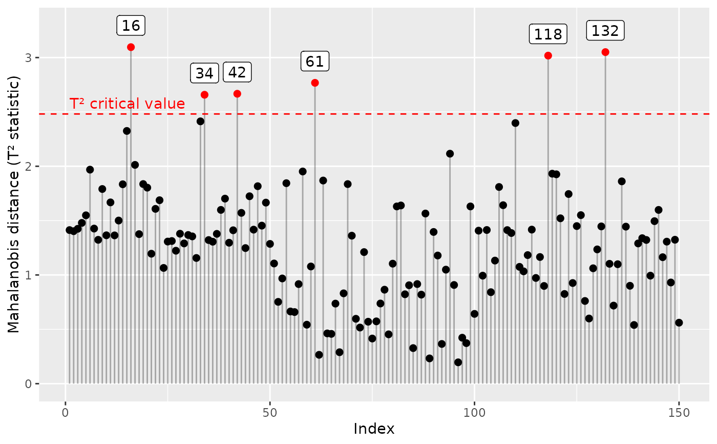
Calculate the T2 statistic for individual points

Calculate the T2 statistic or Mahalanobis distance for individual points

Usage

outliers(
  x,
  level = 0.95,
  robust = FALSE,
  type = c("t2data", "t2mean", "c2data")
)

plot_outliers(
  x,
  level = 0.95,
  robust = FALSE,
  type = c("t2data", "t2mean", "c2data"),
  labels = NULL
)

Arguments

x: A matrix or data frame with two columns
level: Either coverage probability (for type = "t2data" or "c2data") or confidence level (for type = "t2mean").
robust: If TRUE, then robust estimates of mean and covariance are used
type: what type of statistic should be calculated; can be t2data (for data coverage), t2mean (for difference from a mean) or "c2data" (for coverage calculated with the chi squared statistic)
labels: Optional labels to use on the plot instead of rownames

Value

A data frame with one row per point including the columns d2 (squared mahalanobis distance) t2crit (critical T squared value for the given level), c2crit (critical X squared value for the given level) and is_outlier (logical, whether d2 > t2crit or d2 > c2crit, depending on type).

Details

The function can use a robust estimator of location and scatter using the covMcd function, which uses the Maximum Covariance Determinant (MCD) estimator. Note that while this results in ellipses which are more resistent to outliers, the interpretation slightly changes, as the T2 statistic used is only an approximation in this case. In other words, use it for visualisation and QC, but not for statistical testing.

Examples

library(ggplot2)

pca <- prcomp(iris[, 1:4], scale.=TRUE)
pca_df <- cbind(iris, pca$x)
outlier_stats <- outliers(pca_df[ , c("PC1", "PC2")], level = 0.95)

# use plot_outliers() to directly plot them
plot_outliers(pca_df[ , c("PC1", "PC2")], level = 0.95)