class: center, middle, inverse, title-slide .title[ # Lecture 8: Gene expression analysis ] .subtitle[ ## BE_22 Bioinformatics SS 21 ] .author[ ### January Weiner ] .date[ ### 2024-06-10 ] --- <!-- class:empty-slide,myinverse background-image:url(images/arnolfini.jpg) --> ## Plan for today * Gene expression analysis – as an in-depth example of high-throughput analyses --- ## Transcriptomic methods * QPCR: precise, low-throughput * Nanostring: precise, mid-throughput (~ 500-1000 genes) * Microarray: less exact, high-throughput, pre-defined genes * RNA-Seq: very flexible, less exact, high-throughput --- ## QC – quality control * Method-dependent quality measures * aligned reads * duplications * intron / exon binding * Y chromosome binding * adapter content * Bias? Clustering? --- ## (Demo) Example RNA-Seq QC Document derived using the `multiQC` package can be retrieved [here](multiqc.all_samples.all_mates.qc_report.html) --- ## The GSE156063 data set <table> <thead> <tr> <th style="text-align:left;"> Col </th> <th style="text-align:left;"> Class </th> <th style="text-align:right;"> NAs </th> <th style="text-align:right;"> unique </th> <th style="text-align:left;"> Summary </th> </tr> </thead> <tbody> <tr> <td style="text-align:left;"> label </td> <td style="text-align:left;"> <chr> </td> <td style="text-align:right;"> 0 </td> <td style="text-align:right;"> 234 </td> <td style="text-align:left;"> All values unique </td> </tr> <tr> <td style="text-align:left;"> filename </td> <td style="text-align:left;"> <chr> </td> <td style="text-align:right;"> 0 </td> <td style="text-align:right;"> 234 </td> <td style="text-align:left;"> All values unique </td> </tr> <tr> <td style="text-align:left;"> md5 </td> <td style="text-align:left;"> <chr> </td> <td style="text-align:right;"> 0 </td> <td style="text-align:right;"> 234 </td> <td style="text-align:left;"> All values unique </td> </tr> <tr> <td style="text-align:left;"> replicate </td> <td style="text-align:left;"> <int> </td> <td style="text-align:right;"> 0 </td> <td style="text-align:right;"> 1 </td> <td style="text-align:left;"> 1 </td> </tr> <tr> <td style="text-align:left;"> title </td> <td style="text-align:left;"> <chr> </td> <td style="text-align:right;"> 0 </td> <td style="text-align:right;"> 234 </td> <td style="text-align:left;"> All values unique </td> </tr> <tr> <td style="text-align:left;"> geo_accession </td> <td style="text-align:left;"> <chr> </td> <td style="text-align:right;"> 0 </td> <td style="text-align:right;"> 234 </td> <td style="text-align:left;"> All values unique </td> </tr> <tr> <td style="text-align:left;"> age </td> <td style="text-align:left;"> <dbl> </td> <td style="text-align:right;"> 0 </td> <td style="text-align:right;"> 68 </td> <td style="text-align:left;"> 20.0 [40.0 <50.5> 65.0] 89.0 </td> </tr> <tr> <td style="text-align:left;"> disease_state </td> <td style="text-align:left;"> <chr> </td> <td style="text-align:right;"> 0 </td> <td style="text-align:right;"> 3 </td> <td style="text-align:left;"> no virus: 100, SC2: 93, other virus: 41 </td> </tr> <tr> <td style="text-align:left;"> gender </td> <td style="text-align:left;"> <chr> </td> <td style="text-align:right;"> 0 </td> <td style="text-align:right;"> 2 </td> <td style="text-align:left;"> F: 124, M: 110 </td> </tr> <tr> <td style="text-align:left;"> group </td> <td style="text-align:left;"> <chr> </td> <td style="text-align:right;"> 0 </td> <td style="text-align:right;"> 3 </td> <td style="text-align:left;"> no: 100, SC2: 93, other: 41 </td> </tr> <tr> <td style="text-align:left;"> sizeFactor </td> <td style="text-align:left;"> <dbl> </td> <td style="text-align:right;"> 0 </td> <td style="text-align:right;"> 234 </td> <td style="text-align:left;"> 0.0754 [0.5049 <1.1083> 2.0840] 7.4839 </td> </tr> <tr> <td style="text-align:left;"> replaceable </td> <td style="text-align:left;"> <lgl> </td> <td style="text-align:right;"> 0 </td> <td style="text-align:right;"> 1 </td> <td style="text-align:left;"> TRUE: 234 FALSE: 0 </td> </tr> </tbody> </table> --- ## The GSE156063 data set <table> <thead> <tr> <th style="text-align:left;"> Col </th> <th style="text-align:left;"> Class </th> <th style="text-align:right;"> NAs </th> <th style="text-align:right;"> unique </th> <th style="text-align:left;"> Summary </th> </tr> </thead> <tbody> <tr> <td style="text-align:left;"> label </td> <td style="text-align:left;"> <chr> </td> <td style="text-align:right;"> 0 </td> <td style="text-align:right;"> 234 </td> <td style="text-align:left;"> All values unique </td> </tr> <tr> <td style="text-align:left;"> filename </td> <td style="text-align:left;"> <chr> </td> <td style="text-align:right;"> 0 </td> <td style="text-align:right;"> 234 </td> <td style="text-align:left;"> All values unique </td> </tr> <tr> <td style="text-align:left;"> md5 </td> <td style="text-align:left;"> <chr> </td> <td style="text-align:right;"> 0 </td> <td style="text-align:right;"> 234 </td> <td style="text-align:left;"> All values unique </td> </tr> <tr> <td style="text-align:left;"> replicate </td> <td style="text-align:left;"> <int> </td> <td style="text-align:right;"> 0 </td> <td style="text-align:right;"> 1 </td> <td style="text-align:left;"> 1 </td> </tr> <tr> <td style="text-align:left;"> title </td> <td style="text-align:left;"> <chr> </td> <td style="text-align:right;"> 0 </td> <td style="text-align:right;"> 234 </td> <td style="text-align:left;"> All values unique </td> </tr> <tr> <td style="text-align:left;"> geo_accession </td> <td style="text-align:left;"> <chr> </td> <td style="text-align:right;"> 0 </td> <td style="text-align:right;"> 234 </td> <td style="text-align:left;"> All values unique </td> </tr> <tr> <td style="text-align:left;font-weight: bold;color: white !important;background-color: #D7261E !important;"> age </td> <td style="text-align:left;font-weight: bold;color: white !important;background-color: #D7261E !important;"> <dbl> </td> <td style="text-align:right;font-weight: bold;color: white !important;background-color: #D7261E !important;"> 0 </td> <td style="text-align:right;font-weight: bold;color: white !important;background-color: #D7261E !important;"> 68 </td> <td style="text-align:left;font-weight: bold;color: white !important;background-color: #D7261E !important;"> 20.0 [40.0 <50.5> 65.0] 89.0 </td> </tr> <tr> <td style="text-align:left;font-weight: bold;color: white !important;background-color: #D7261E !important;"> disease_state </td> <td style="text-align:left;font-weight: bold;color: white !important;background-color: #D7261E !important;"> <chr> </td> <td style="text-align:right;font-weight: bold;color: white !important;background-color: #D7261E !important;"> 0 </td> <td style="text-align:right;font-weight: bold;color: white !important;background-color: #D7261E !important;"> 3 </td> <td style="text-align:left;font-weight: bold;color: white !important;background-color: #D7261E !important;"> no virus: 100, SC2: 93, other virus: 41 </td> </tr> <tr> <td style="text-align:left;font-weight: bold;color: white !important;background-color: #D7261E !important;"> gender </td> <td style="text-align:left;font-weight: bold;color: white !important;background-color: #D7261E !important;"> <chr> </td> <td style="text-align:right;font-weight: bold;color: white !important;background-color: #D7261E !important;"> 0 </td> <td style="text-align:right;font-weight: bold;color: white !important;background-color: #D7261E !important;"> 2 </td> <td style="text-align:left;font-weight: bold;color: white !important;background-color: #D7261E !important;"> F: 124, M: 110 </td> </tr> <tr> <td style="text-align:left;font-weight: bold;color: white !important;background-color: #D7261E !important;"> group </td> <td style="text-align:left;font-weight: bold;color: white !important;background-color: #D7261E !important;"> <chr> </td> <td style="text-align:right;font-weight: bold;color: white !important;background-color: #D7261E !important;"> 0 </td> <td style="text-align:right;font-weight: bold;color: white !important;background-color: #D7261E !important;"> 3 </td> <td style="text-align:left;font-weight: bold;color: white !important;background-color: #D7261E !important;"> no: 100, SC2: 93, other: 41 </td> </tr> <tr> <td style="text-align:left;"> sizeFactor </td> <td style="text-align:left;"> <dbl> </td> <td style="text-align:right;"> 0 </td> <td style="text-align:right;"> 234 </td> <td style="text-align:left;"> 0.0754 [0.5049 <1.1083> 2.0840] 7.4839 </td> </tr> <tr> <td style="text-align:left;"> replaceable </td> <td style="text-align:left;"> <lgl> </td> <td style="text-align:right;"> 0 </td> <td style="text-align:right;"> 1 </td> <td style="text-align:left;"> TRUE: 234 FALSE: 0 </td> </tr> </tbody> </table> --- How do the count data look like? <table> <thead> <tr> <th style="text-align:left;"> </th> <th style="text-align:right;"> RR057e_00037 </th> <th style="text-align:right;"> RR057e_00039 </th> <th style="text-align:right;"> RR057e_00042 </th> <th style="text-align:right;"> RR057e_00047 </th> <th style="text-align:right;"> RR057e_00049 </th> <th style="text-align:right;"> RR057e_00051 </th> <th style="text-align:left;"> ... </th> </tr> </thead> <tbody> <tr> <td style="text-align:left;"> ENSG00000000003 </td> <td style="text-align:right;"> 40 </td> <td style="text-align:right;"> 20 </td> <td style="text-align:right;"> 488 </td> <td style="text-align:right;"> 48 </td> <td style="text-align:right;"> 8 </td> <td style="text-align:right;"> 143 </td> <td style="text-align:left;"> ... </td> </tr> <tr> <td style="text-align:left;"> ENSG00000000419 </td> <td style="text-align:right;"> 18 </td> <td style="text-align:right;"> 43 </td> <td style="text-align:right;"> 163 </td> <td style="text-align:right;"> 9 </td> <td style="text-align:right;"> 9 </td> <td style="text-align:right;"> 63 </td> <td style="text-align:left;"> ... </td> </tr> <tr> <td style="text-align:left;"> ENSG00000000457 </td> <td style="text-align:right;"> 19 </td> <td style="text-align:right;"> 36 </td> <td style="text-align:right;"> 264 </td> <td style="text-align:right;"> 30 </td> <td style="text-align:right;"> 13 </td> <td style="text-align:right;"> 115 </td> <td style="text-align:left;"> ... </td> </tr> <tr> <td style="text-align:left;"> ENSG00000000460 </td> <td style="text-align:right;"> 2 </td> <td style="text-align:right;"> 8 </td> <td style="text-align:right;"> 63 </td> <td style="text-align:right;"> 4 </td> <td style="text-align:right;"> 6 </td> <td style="text-align:right;"> 55 </td> <td style="text-align:left;"> ... </td> </tr> <tr> <td style="text-align:left;"> ENSG00000000938 </td> <td style="text-align:right;"> 11 </td> <td style="text-align:right;"> 66 </td> <td style="text-align:right;"> 9 </td> <td style="text-align:right;"> 26 </td> <td style="text-align:right;"> 91 </td> <td style="text-align:right;"> 57 </td> <td style="text-align:left;"> ... </td> </tr> <tr> <td style="text-align:left;"> ENSG00000000971 </td> <td style="text-align:right;"> 74 </td> <td style="text-align:right;"> 32 </td> <td style="text-align:right;"> 236 </td> <td style="text-align:right;"> 24 </td> <td style="text-align:right;"> 8 </td> <td style="text-align:right;"> 73 </td> <td style="text-align:left;"> ... </td> </tr> <tr> <td style="text-align:left;"> ENSG00000001036 </td> <td style="text-align:right;"> 6 </td> <td style="text-align:right;"> 57 </td> <td style="text-align:right;"> 198 </td> <td style="text-align:right;"> 16 </td> <td style="text-align:right;"> 9 </td> <td style="text-align:right;"> 76 </td> <td style="text-align:left;"> ... </td> </tr> <tr> <td style="text-align:left;"> ENSG00000001084 </td> <td style="text-align:right;"> 155 </td> <td style="text-align:right;"> 264 </td> <td style="text-align:right;"> 1799 </td> <td style="text-align:right;"> 43 </td> <td style="text-align:right;"> 25 </td> <td style="text-align:right;"> 472 </td> <td style="text-align:left;"> ... </td> </tr> <tr> <td style="text-align:left;"> ENSG00000001167 </td> <td style="text-align:right;"> 24 </td> <td style="text-align:right;"> 18 </td> <td style="text-align:right;"> 135 </td> <td style="text-align:right;"> 26 </td> <td style="text-align:right;"> 40 </td> <td style="text-align:right;"> 101 </td> <td style="text-align:left;"> ... </td> </tr> <tr> <td style="text-align:left;"> ENSG00000001460 </td> <td style="text-align:right;"> 88 </td> <td style="text-align:right;"> 20 </td> <td style="text-align:right;"> 449 </td> <td style="text-align:right;"> 7 </td> <td style="text-align:right;"> 6 </td> <td style="text-align:right;"> 165 </td> <td style="text-align:left;"> ... </td> </tr> </tbody> </table> --- # QC using PCA Dimension reduction with PCA allows us to see batch effects and also have a first preliminary look at the data. --- .pull-left[ ### Before PCA: <!-- --> Correlation between x and y = 0.66 ] .pull-right[ ### After PCA: <!-- --> Correlation between PC1 and PC2 = -0.00 ] --- .pull-left[ ### Before PCA: <!-- --> Correlation between x and y = 0.84 ] .pull-right[ ### After PCA: <!-- --> Correlation between PC1 and PC2 = 0.00 ] --- .pull-left[ ### Before PCA: <!-- --> ] .pull-right[ ### After PCA: <!-- --> ] --- <div class="plotly html-widget html-fill-item-overflow-hidden html-fill-item" id="htmlwidget-82afad98a1394dd2ee0a" style="width:864px;height:576px;"></div> <script type="application/json" data-for="htmlwidget-82afad98a1394dd2ee0a">{"x":{"visdat":{"331d43821c198":["function () ","plotlyVisDat"],"331d435a96702":["function () ","data"],"331d44780db2f":["function () ","data"],"331d4352c2db4":["function () ","data"]},"cur_data":"331d4352c2db4","attrs":{"331d43821c198":{"mode":"markers","x":[-16.640000000000001,0.1268,-12.07,2.5310000000000001,12.539999999999999,-7.4980000000000002,-17.440000000000001,-0.8337,18.789999999999999,11.94,-1.3879999999999999,11.1,-1.9910000000000001,29.050000000000001,3.327,-3.2519999999999998,-5.4909999999999997,-12.789999999999999,-11.75,-7.8040000000000003,-4.3120000000000003,20.629999999999999,-5.508,-9.0359999999999996,-0.55700000000000005,-15.550000000000001,17.350000000000001,1.413,1.0069999999999999,7.9870000000000001,3.6509999999999998,2.1269999999999998,18.039999999999999,12.109999999999999,-7.0220000000000002,7.3399999999999999,-8.2899999999999991,21.829999999999998,-6.4080000000000004,7.4329999999999998,19.620000000000001,31.300000000000001,-7.2229999999999999,32.5,-6.6689999999999996,-18.289999999999999,13.970000000000001,-10.119999999999999,30.969999999999999,-7.5780000000000003,-4.3559999999999999,-18.98,-3.1869999999999998,26.510000000000002,23.260000000000002,19.239999999999998,-3.9820000000000002,5.8819999999999997,-15.029999999999999,20.739999999999998,-0.73609999999999998,-21.91,4.2190000000000003,-5.2169999999999996,0.21360000000000001,-17.510000000000002,-1.3009999999999999,-3.9620000000000002,-16.82,-9.3160000000000007,6.1429999999999998,16.32,12.029999999999999,-20.789999999999999,-16.789999999999999,-14.69,22.5,-7.915,1.056,-7.657,-11.15,4.7279999999999998,-22.93,-6.1980000000000004,16.789999999999999,17.91,19.289999999999999,5.6890000000000001,15.02,23.949999999999999,12.49,-13.51,1.2969999999999999,26.010000000000002,-13.529999999999999,16.57,11.4,21.25,21.18,1.6439999999999999,-19,23.399999999999999,1.653,12.56,15.199999999999999,-0.078310000000000005,-16.73,-6.8940000000000001,16.760000000000002,8.1790000000000003,28.84,0.7248,17.32,23.41,25.16,0.52359999999999995,-11.67,-7.2889999999999997,-15.720000000000001,14.640000000000001,18.190000000000001,9.2100000000000009,-9.3190000000000008,-5.5709999999999997,-0.38740000000000002,-6.8929999999999998,-10.91,-4.2720000000000002,-5.8680000000000003,-22.02,-11.6,-6.6909999999999998,-14.99,-8.6950000000000003,-9.5250000000000004,-9.8100000000000005,-11.08,-2.1070000000000002,-15.710000000000001,-3.9100000000000001,-0.6552,-4.2089999999999996,-11.92,-11.32,5.9930000000000003,-6.5140000000000002,-1.446,-3.5390000000000001,-10.800000000000001,-13.93,0.83179999999999998,-15.84,12.99,-5.2439999999999998,16.649999999999999,-3.6669999999999998,24.559999999999999,-16.960000000000001,-6.0700000000000003,14.66,-7.181,-8.2970000000000006,-4.2629999999999999,-2.952,-7.5279999999999996,-0.015800000000000002,-6.6479999999999997,13.970000000000001,1.645,-2.3439999999999999,4.2619999999999996,22.84,-12.369999999999999,-3.2970000000000002,-9.0399999999999991,-11.84,-1.744,1.2669999999999999,2.0409999999999999,-3.4820000000000002,-1.6299999999999999,-4.798,-4.7069999999999999,-0.72860000000000003,-1.7050000000000001,-2.0710000000000002,-4.5460000000000003,10.369999999999999,0.92420000000000002,10.869999999999999,31.07,-1.0189999999999999,17.640000000000001,8.2560000000000002,-9.6460000000000008,-20.460000000000001,-11.800000000000001,12.220000000000001,-17.809999999999999,-1.925,0.99419999999999997,-8.6509999999999998,-16.050000000000001,-5.4770000000000003,-0.45240000000000002,-7.657,-6.952,4.242,-11.59,-2.4239999999999999,6.1299999999999999,1.0640000000000001,5.6849999999999996,19.829999999999998,6.4539999999999997,16.120000000000001,-10.039999999999999,-12.19,-8.9870000000000001,-6.3840000000000003,8.4960000000000004,1.8560000000000001,-12.24,-12.470000000000001,9.843,-11.9,-11.210000000000001,-13.58,-19.800000000000001,-17.210000000000001,-12.82,-12.32,-11.26,-14.24],"y":[-19.09,-19.760000000000002,-9.0950000000000006,-25.449999999999999,-19.100000000000001,-9.4920000000000009,-0.5413,1.911,-7.4219999999999997,0.53549999999999998,4.3769999999999998,6.2290000000000001,6.9290000000000003,-5.0099999999999998,8.2439999999999998,3.6379999999999999,4.0650000000000004,-12.69,-0.30609999999999998,5.7000000000000002,8.5530000000000008,4.032,-12.99,-16.960000000000001,-9.3599999999999994,-0.66369999999999996,-8.1479999999999997,0.51639999999999997,-22.350000000000001,1.9770000000000001,-7.9089999999999998,-0.1145,6.9740000000000002,0.074260000000000007,-13.65,-0.3352,5.194,5.8010000000000002,9.1479999999999997,9.9870000000000001,9.2360000000000007,-9.4870000000000001,9.1110000000000007,-6.0490000000000004,5.04,0.0141,3.1349999999999998,1.3680000000000001,-5.6479999999999997,-7.1390000000000002,7.2060000000000004,5.6509999999999998,2.1749999999999998,-5.2530000000000001,5.3170000000000002,10.68,6.1340000000000003,6.7359999999999998,4.1820000000000004,2.746,9.8379999999999992,-2.4540000000000002,-4.0350000000000001,-10.73,-12.960000000000001,-10.710000000000001,-5.907,-8.4749999999999996,3.7400000000000002,6.1139999999999999,9.6850000000000005,8.4610000000000003,3.633,1.101,3.8420000000000001,-1.6619999999999999,1.1259999999999999,2.8650000000000002,-4.6440000000000001,-9.5619999999999994,-0.16209999999999999,12.359999999999999,2.7909999999999999,8.8650000000000002,10.66,-8.0449999999999999,-15.23,-0.28489999999999999,3.1219999999999999,3.137,8.6229999999999993,0.73419999999999996,-6.032,-1.7250000000000001,2.2010000000000001,5.8559999999999999,11.73,4.2169999999999996,-3.7749999999999999,7.9379999999999997,2.758,-2.746,2.4119999999999999,6.4059999999999997,11.130000000000001,6.399,4.7990000000000004,1.375,4.6319999999999997,0.52210000000000001,-13.5,-9.4299999999999997,2.2400000000000002,-15.84,-5.9219999999999997,-20.690000000000001,-7.25,-8.4870000000000001,-18.239999999999998,1.097,4.1660000000000004,-24.219999999999999,-3.3530000000000002,-10.470000000000001,-15.49,4.593,-4.657,9.0969999999999995,-1.387,-10.65,7.5149999999999997,-11.800000000000001,-8.5660000000000007,-21.09,8.4440000000000008,-7.016,-10.91,-16.649999999999999,6.6559999999999997,10.220000000000001,-16.210000000000001,7.0599999999999996,5.7969999999999997,8.2650000000000006,-1.4610000000000001,-1.448,5.9169999999999998,2.8849999999999998,-0.63849999999999996,-3.4489999999999998,7.1520000000000001,4.6769999999999996,3.7629999999999999,7.4299999999999997,8.5150000000000006,1.05,-1.6850000000000001,-11.6,1.5680000000000001,-4.2409999999999997,-9.4399999999999995,10.08,0.25580000000000003,4.7149999999999999,2.8490000000000002,7.4749999999999996,5.8890000000000002,4.4480000000000004,5.0970000000000004,3.3929999999999998,4.3559999999999999,-2.0470000000000002,0.42849999999999999,-0.27579999999999999,3.2639999999999998,3.2570000000000001,6.8460000000000001,5.407,1.6000000000000001,-0.034450000000000001,-8.2929999999999993,-1.554,2.7599999999999998,2.8820000000000001,-2.169,2.8300000000000001,1.369,3.589,-4.6689999999999996,-2.081,-16.489999999999998,-16.899999999999999,11.220000000000001,-0.90839999999999999,6.1970000000000001,1.9730000000000001,-2.6949999999999998,8.8420000000000005,-0.36349999999999999,7.8520000000000003,-0.316,6.6369999999999996,-16.140000000000001,8.3529999999999998,1.6519999999999999,7.2720000000000002,3.125,10.199999999999999,0.51419999999999999,1.2,-1.7450000000000001,-8.9299999999999997,8.0410000000000004,9.6600000000000001,8.4629999999999992,8.4390000000000001,8.5449999999999999,-1.4039999999999999,9.5879999999999992,-1.2669999999999999,-9.2680000000000007,6.0679999999999996,2.6789999999999998,7.0030000000000001,12.91,5.4379999999999997,9.3209999999999997,4.3650000000000002,-0.97150000000000003,4.9960000000000004,2.4060000000000001,9.1769999999999996,10.039999999999999,8.6869999999999994],"hovertext":["group: other<br />gender: F<br />disease_state: other virus<br />age: 67<br />plotlyID: ID1","group: no<br />gender: M<br />disease_state: no virus<br />age: 42<br />plotlyID: ID2","group: no<br />gender: F<br />disease_state: no virus<br />age: 38<br />plotlyID: ID3","group: other<br />gender: M<br />disease_state: other virus<br />age: 45<br />plotlyID: ID4","group: no<br />gender: M<br />disease_state: no virus<br />age: 60<br />plotlyID: ID5","group: no<br />gender: M<br />disease_state: no virus<br />age: 75<br />plotlyID: ID6","group: no<br />gender: F<br />disease_state: no virus<br />age: 64<br />plotlyID: ID7","group: no<br />gender: M<br />disease_state: no virus<br />age: 66<br />plotlyID: ID8","group: other<br />gender: M<br />disease_state: other virus<br />age: 73<br />plotlyID: ID9","group: no<br />gender: F<br />disease_state: no virus<br />age: 82<br />plotlyID: ID10","group: no<br />gender: F<br />disease_state: no virus<br />age: 33<br />plotlyID: ID11","group: no<br />gender: M<br />disease_state: no virus<br />age: 57<br />plotlyID: ID12","group: no<br />gender: F<br />disease_state: no virus<br />age: 34<br />plotlyID: ID13","group: no<br />gender: F<br />disease_state: no virus<br />age: 54<br />plotlyID: ID14","group: no<br />gender: M<br />disease_state: no virus<br />age: 81<br />plotlyID: ID15","group: no<br />gender: F<br />disease_state: no virus<br />age: 38<br />plotlyID: ID16","group: no<br />gender: M<br />disease_state: no virus<br />age: 42<br />plotlyID: ID17","group: no<br />gender: F<br />disease_state: no virus<br />age: 66<br />plotlyID: ID18","group: no<br />gender: F<br />disease_state: no virus<br />age: 72<br />plotlyID: ID19","group: no<br />gender: F<br />disease_state: no virus<br />age: 29<br />plotlyID: ID20","group: no<br />gender: F<br />disease_state: no virus<br />age: 66<br />plotlyID: ID21","group: other<br />gender: M<br />disease_state: other virus<br />age: 40<br />plotlyID: ID22","group: no<br />gender: M<br />disease_state: no virus<br />age: 70<br />plotlyID: ID23","group: no<br />gender: F<br />disease_state: no virus<br />age: 38<br />plotlyID: ID24","group: no<br />gender: F<br />disease_state: no virus<br />age: 73<br />plotlyID: ID25","group: no<br />gender: M<br />disease_state: no virus<br />age: 88<br />plotlyID: ID26","group: no<br />gender: F<br />disease_state: no virus<br />age: 76<br />plotlyID: ID27","group: other<br />gender: F<br />disease_state: other virus<br />age: 34<br />plotlyID: ID28","group: other<br />gender: F<br />disease_state: other virus<br />age: 32<br />plotlyID: ID29","group: other<br />gender: F<br />disease_state: other virus<br />age: 38<br />plotlyID: ID30","group: no<br />gender: M<br />disease_state: no virus<br />age: 74<br />plotlyID: ID31","group: no<br />gender: F<br />disease_state: no virus<br />age: 44<br />plotlyID: ID32","group: no<br />gender: M<br />disease_state: no virus<br />age: 64<br />plotlyID: ID33","group: no<br />gender: M<br />disease_state: no virus<br />age: 36<br />plotlyID: ID34","group: no<br />gender: F<br />disease_state: no virus<br />age: 72<br />plotlyID: ID35","group: other<br />gender: F<br />disease_state: other virus<br />age: 21<br />plotlyID: ID36","group: SC2<br />gender: M<br />disease_state: SC2<br />age: 46<br />plotlyID: ID37","group: other<br />gender: F<br />disease_state: other virus<br />age: 30<br />plotlyID: ID38","group: no<br />gender: M<br />disease_state: no virus<br />age: 56<br />plotlyID: ID39","group: no<br />gender: M<br />disease_state: no virus<br />age: 65<br />plotlyID: ID40","group: no<br />gender: F<br />disease_state: no virus<br />age: 53<br />plotlyID: ID41","group: no<br />gender: F<br />disease_state: no virus<br />age: 82<br />plotlyID: ID42","group: no<br />gender: M<br />disease_state: no virus<br />age: 71<br />plotlyID: ID43","group: other<br />gender: M<br />disease_state: other virus<br />age: 61<br />plotlyID: ID44","group: no<br />gender: F<br />disease_state: no virus<br />age: 47<br />plotlyID: ID45","group: no<br />gender: M<br />disease_state: no virus<br />age: 48<br />plotlyID: ID46","group: other<br />gender: M<br />disease_state: other virus<br />age: 25<br />plotlyID: ID47","group: no<br />gender: F<br />disease_state: no virus<br />age: 62<br />plotlyID: ID48","group: no<br />gender: M<br />disease_state: no virus<br />age: 39<br />plotlyID: ID49","group: no<br />gender: M<br />disease_state: no virus<br />age: 74<br />plotlyID: ID50","group: no<br />gender: F<br />disease_state: no virus<br />age: 64<br />plotlyID: ID51","group: no<br />gender: F<br />disease_state: no virus<br />age: 72<br />plotlyID: ID52","group: other<br />gender: M<br />disease_state: other virus<br />age: 62<br />plotlyID: ID53","group: other<br />gender: F<br />disease_state: other virus<br />age: 46<br />plotlyID: ID54","group: no<br />gender: F<br />disease_state: no virus<br />age: 44<br />plotlyID: ID55","group: other<br />gender: F<br />disease_state: other virus<br />age: 47<br />plotlyID: ID56","group: other<br />gender: F<br />disease_state: other virus<br />age: 33<br />plotlyID: ID57","group: no<br />gender: M<br />disease_state: no virus<br />age: 63<br />plotlyID: ID58","group: no<br />gender: M<br />disease_state: no virus<br />age: 63<br />plotlyID: ID59","group: other<br />gender: M<br />disease_state: other virus<br />age: 71<br />plotlyID: ID60","group: other<br />gender: M<br />disease_state: other virus<br />age: 51<br />plotlyID: ID61","group: no<br />gender: M<br />disease_state: no virus<br />age: 45<br />plotlyID: ID62","group: no<br />gender: M<br />disease_state: no virus<br />age: 44<br />plotlyID: ID63","group: no<br />gender: F<br />disease_state: no virus<br />age: 73<br />plotlyID: ID64","group: no<br />gender: M<br />disease_state: no virus<br />age: 51<br />plotlyID: ID65","group: no<br />gender: F<br />disease_state: no virus<br />age: 52<br />plotlyID: ID66","group: no<br />gender: M<br />disease_state: no virus<br />age: 67<br />plotlyID: ID67","group: no<br />gender: F<br />disease_state: no virus<br />age: 85<br />plotlyID: ID68","group: no<br />gender: F<br />disease_state: no virus<br />age: 64<br />plotlyID: ID69","group: no<br />gender: F<br />disease_state: no virus<br />age: 83<br />plotlyID: ID70","group: no<br />gender: F<br />disease_state: no virus<br />age: 76<br />plotlyID: ID71","group: no<br />gender: F<br />disease_state: no virus<br />age: 44<br />plotlyID: ID72","group: no<br />gender: M<br />disease_state: no virus<br />age: 42<br />plotlyID: ID73","group: no<br />gender: F<br />disease_state: no virus<br />age: 59<br />plotlyID: ID74","group: no<br />gender: F<br />disease_state: no virus<br />age: 57<br />plotlyID: ID75","group: other<br />gender: F<br />disease_state: other virus<br />age: 35<br />plotlyID: ID76","group: no<br />gender: M<br />disease_state: no virus<br />age: 71<br />plotlyID: ID77","group: no<br />gender: M<br />disease_state: no virus<br />age: 77<br />plotlyID: ID78","group: no<br />gender: F<br />disease_state: no virus<br />age: 35<br />plotlyID: ID79","group: no<br />gender: F<br />disease_state: no virus<br />age: 24<br />plotlyID: ID80","group: no<br />gender: F<br />disease_state: no virus<br />age: 46<br />plotlyID: ID81","group: no<br />gender: M<br />disease_state: no virus<br />age: 73<br />plotlyID: ID82","group: no<br />gender: F<br />disease_state: no virus<br />age: 77<br />plotlyID: ID83","group: other<br />gender: F<br />disease_state: other virus<br />age: 34<br />plotlyID: ID84","group: no<br />gender: F<br />disease_state: no virus<br />age: 65<br />plotlyID: ID85","group: no<br />gender: M<br />disease_state: no virus<br />age: 72<br />plotlyID: ID86","group: no<br />gender: M<br />disease_state: no virus<br />age: 45<br />plotlyID: ID87","group: no<br />gender: F<br />disease_state: no virus<br />age: 37<br />plotlyID: ID88","group: other<br />gender: F<br />disease_state: other virus<br />age: 34<br />plotlyID: ID89","group: other<br />gender: M<br />disease_state: other virus<br />age: 86<br />plotlyID: ID90","group: other<br />gender: F<br />disease_state: other virus<br />age: 67<br />plotlyID: ID91","group: other<br />gender: M<br />disease_state: other virus<br />age: 48<br />plotlyID: ID92","group: other<br />gender: M<br />disease_state: other virus<br />age: 69<br />plotlyID: ID93","group: other<br />gender: M<br />disease_state: other virus<br />age: 69<br />plotlyID: ID94","group: no<br />gender: F<br />disease_state: no virus<br />age: 82<br />plotlyID: ID95","group: no<br />gender: F<br />disease_state: no virus<br />age: 70<br />plotlyID: ID96","group: no<br />gender: F<br />disease_state: no virus<br />age: 65<br />plotlyID: ID97","group: no<br />gender: M<br />disease_state: no virus<br />age: 78<br />plotlyID: ID98","group: other<br />gender: M<br />disease_state: other virus<br />age: 82<br />plotlyID: ID99","group: no<br />gender: M<br />disease_state: no virus<br />age: 67<br />plotlyID: ID100","group: no<br />gender: F<br />disease_state: no virus<br />age: 44<br />plotlyID: ID101","group: no<br />gender: M<br />disease_state: no virus<br />age: 52<br />plotlyID: ID102","group: no<br />gender: F<br />disease_state: no virus<br />age: 62<br />plotlyID: ID103","group: other<br />gender: M<br />disease_state: other virus<br />age: 29<br />plotlyID: ID104","group: other<br />gender: M<br />disease_state: other virus<br />age: 40<br />plotlyID: ID105","group: other<br />gender: M<br />disease_state: other virus<br />age: 75<br />plotlyID: ID106","group: no<br />gender: M<br />disease_state: no virus<br />age: 64<br />plotlyID: ID107","group: other<br />gender: M<br />disease_state: other virus<br />age: 25<br />plotlyID: ID108","group: other<br />gender: M<br />disease_state: other virus<br />age: 89<br />plotlyID: ID109","group: no<br />gender: M<br />disease_state: no virus<br />age: 49<br />plotlyID: ID110","group: other<br />gender: M<br />disease_state: other virus<br />age: 35<br />plotlyID: ID111","group: no<br />gender: F<br />disease_state: no virus<br />age: 41<br />plotlyID: ID112","group: other<br />gender: M<br />disease_state: other virus<br />age: 55<br />plotlyID: ID113","group: other<br />gender: F<br />disease_state: other virus<br />age: 79<br />plotlyID: ID114","group: other<br />gender: F<br />disease_state: other virus<br />age: 57<br />plotlyID: ID115","group: other<br />gender: F<br />disease_state: other virus<br />age: 42<br />plotlyID: ID116","group: no<br />gender: F<br />disease_state: no virus<br />age: 60<br />plotlyID: ID117","group: no<br />gender: M<br />disease_state: no virus<br />age: 89<br />plotlyID: ID118","group: no<br />gender: F<br />disease_state: no virus<br />age: 59<br />plotlyID: ID119","group: other<br />gender: F<br />disease_state: other virus<br />age: 42<br />plotlyID: ID120","group: other<br />gender: F<br />disease_state: other virus<br />age: 40<br />plotlyID: ID121","group: other<br />gender: M<br />disease_state: other virus<br />age: 85<br />plotlyID: ID122","group: no<br />gender: F<br />disease_state: no virus<br />age: 41<br />plotlyID: ID123","group: SC2<br />gender: M<br />disease_state: SC2<br />age: 40<br />plotlyID: ID124","group: SC2<br />gender: M<br />disease_state: SC2<br />age: 27<br />plotlyID: ID125","group: SC2<br />gender: F<br />disease_state: SC2<br />age: 43<br />plotlyID: ID126","group: SC2<br />gender: F<br />disease_state: SC2<br />age: 30<br />plotlyID: ID127","group: SC2<br />gender: M<br />disease_state: SC2<br />age: 74<br />plotlyID: ID128","group: SC2<br />gender: F<br />disease_state: SC2<br />age: 55<br />plotlyID: ID129","group: SC2<br />gender: F<br />disease_state: SC2<br />age: 40<br />plotlyID: ID130","group: SC2<br />gender: F<br />disease_state: SC2<br />age: 35<br />plotlyID: ID131","group: SC2<br />gender: F<br />disease_state: SC2<br />age: 63<br />plotlyID: ID132","group: SC2<br />gender: M<br />disease_state: SC2<br />age: 58<br />plotlyID: ID133","group: SC2<br />gender: M<br />disease_state: SC2<br />age: 20<br />plotlyID: ID134","group: SC2<br />gender: F<br />disease_state: SC2<br />age: 51<br />plotlyID: ID135","group: SC2<br />gender: F<br />disease_state: SC2<br />age: 35<br />plotlyID: ID136","group: SC2<br />gender: F<br />disease_state: SC2<br />age: 38<br />plotlyID: ID137","group: SC2<br />gender: M<br />disease_state: SC2<br />age: 54<br />plotlyID: ID138","group: SC2<br />gender: F<br />disease_state: SC2<br />age: 32<br />plotlyID: ID139","group: SC2<br />gender: M<br />disease_state: SC2<br />age: 32<br />plotlyID: ID140","group: SC2<br />gender: M<br />disease_state: SC2<br />age: 82<br />plotlyID: ID141","group: SC2<br />gender: F<br />disease_state: SC2<br />age: 32<br />plotlyID: ID142","group: SC2<br />gender: M<br />disease_state: SC2<br />age: 28<br />plotlyID: ID143","group: SC2<br />gender: M<br />disease_state: SC2<br />age: 55<br />plotlyID: ID144","group: SC2<br />gender: F<br />disease_state: SC2<br />age: 67<br />plotlyID: ID145","group: SC2<br />gender: F<br />disease_state: SC2<br />age: 58<br />plotlyID: ID146","group: SC2<br />gender: M<br />disease_state: SC2<br />age: 41<br />plotlyID: ID147","group: SC2<br />gender: F<br />disease_state: SC2<br />age: 36<br />plotlyID: ID148","group: SC2<br />gender: M<br />disease_state: SC2<br />age: 68<br />plotlyID: ID149","group: SC2<br />gender: F<br />disease_state: SC2<br />age: 69<br />plotlyID: ID150","group: SC2<br />gender: F<br />disease_state: SC2<br />age: 34<br />plotlyID: ID151","group: SC2<br />gender: F<br />disease_state: SC2<br />age: 64<br />plotlyID: ID152","group: SC2<br />gender: M<br />disease_state: SC2<br />age: 46<br />plotlyID: ID153","group: other<br />gender: M<br />disease_state: other virus<br />age: 44<br />plotlyID: ID154","group: no<br />gender: M<br />disease_state: no virus<br />age: 33<br />plotlyID: ID155","group: no<br />gender: M<br />disease_state: no virus<br />age: 41<br />plotlyID: ID156","group: other<br />gender: F<br />disease_state: other virus<br />age: 71<br />plotlyID: ID157","group: no<br />gender: M<br />disease_state: no virus<br />age: 54<br />plotlyID: ID158","group: SC2<br />gender: M<br />disease_state: SC2<br />age: 43<br />plotlyID: ID159","group: SC2<br />gender: F<br />disease_state: SC2<br />age: 44<br />plotlyID: ID160","group: SC2<br />gender: F<br />disease_state: SC2<br />age: 44<br />plotlyID: ID161","group: SC2<br />gender: F<br />disease_state: SC2<br />age: 62<br />plotlyID: ID162","group: SC2<br />gender: M<br />disease_state: SC2<br />age: 35<br />plotlyID: ID163","group: SC2<br />gender: F<br />disease_state: SC2<br />age: 44<br />plotlyID: ID164","group: SC2<br />gender: F<br />disease_state: SC2<br />age: 57<br />plotlyID: ID165","group: SC2<br />gender: F<br />disease_state: SC2<br />age: 33<br />plotlyID: ID166","group: SC2<br />gender: M<br />disease_state: SC2<br />age: 62<br />plotlyID: ID167","group: no<br />gender: M<br />disease_state: no virus<br />age: 50<br />plotlyID: ID168","group: SC2<br />gender: F<br />disease_state: SC2<br />age: 26<br />plotlyID: ID169","group: SC2<br />gender: M<br />disease_state: SC2<br />age: 29<br />plotlyID: ID170","group: SC2<br />gender: M<br />disease_state: SC2<br />age: 34<br />plotlyID: ID171","group: SC2<br />gender: M<br />disease_state: SC2<br />age: 24<br />plotlyID: ID172","group: SC2<br />gender: F<br />disease_state: SC2<br />age: 47<br />plotlyID: ID173","group: SC2<br />gender: F<br />disease_state: SC2<br />age: 63<br />plotlyID: ID174","group: no<br />gender: F<br />disease_state: no virus<br />age: 63<br />plotlyID: ID175","group: SC2<br />gender: F<br />disease_state: SC2<br />age: 42<br />plotlyID: ID176","group: SC2<br />gender: F<br />disease_state: SC2<br />age: 27<br />plotlyID: ID177","group: SC2<br />gender: F<br />disease_state: SC2<br />age: 20<br />plotlyID: ID178","group: SC2<br />gender: M<br />disease_state: SC2<br />age: 29<br />plotlyID: ID179","group: SC2<br />gender: F<br />disease_state: SC2<br />age: 76<br />plotlyID: ID180","group: SC2<br />gender: M<br />disease_state: SC2<br />age: 46.8915662650602<br />plotlyID: ID181","group: SC2<br />gender: M<br />disease_state: SC2<br />age: 46.8915662650602<br />plotlyID: ID182","group: SC2<br />gender: F<br />disease_state: SC2<br />age: 46.8915662650602<br />plotlyID: ID183","group: SC2<br />gender: F<br />disease_state: SC2<br />age: 46.8915662650602<br />plotlyID: ID184","group: SC2<br />gender: M<br />disease_state: SC2<br />age: 46.8915662650602<br />plotlyID: ID185","group: SC2<br />gender: F<br />disease_state: SC2<br />age: 46.8915662650602<br />plotlyID: ID186","group: SC2<br />gender: M<br />disease_state: SC2<br />age: 46.8915662650602<br />plotlyID: ID187","group: SC2<br />gender: M<br />disease_state: SC2<br />age: 46.8915662650602<br />plotlyID: ID188","group: SC2<br />gender: M<br />disease_state: SC2<br />age: 46.8915662650602<br />plotlyID: ID189","group: SC2<br />gender: M<br />disease_state: SC2<br />age: 46.8915662650602<br />plotlyID: ID190","group: SC2<br />gender: M<br />disease_state: SC2<br />age: 53<br />plotlyID: ID191","group: SC2<br />gender: M<br />disease_state: SC2<br />age: 41<br />plotlyID: ID192","group: SC2<br />gender: F<br />disease_state: SC2<br />age: 62<br />plotlyID: ID193","group: SC2<br />gender: F<br />disease_state: SC2<br />age: 43<br />plotlyID: ID194","group: SC2<br />gender: M<br />disease_state: SC2<br />age: 62<br />plotlyID: ID195","group: no<br />gender: M<br />disease_state: no virus<br />age: 53<br />plotlyID: ID196","group: no<br />gender: F<br />disease_state: no virus<br />age: 54<br />plotlyID: ID197","group: no<br />gender: F<br />disease_state: no virus<br />age: 52<br />plotlyID: ID198","group: no<br />gender: M<br />disease_state: no virus<br />age: 53<br />plotlyID: ID199","group: no<br />gender: F<br />disease_state: no virus<br />age: 46<br />plotlyID: ID200","group: no<br />gender: M<br />disease_state: no virus<br />age: 57.2020202020202<br />plotlyID: ID201","group: SC2<br />gender: F<br />disease_state: SC2<br />age: 44<br />plotlyID: ID202","group: SC2<br />gender: M<br />disease_state: SC2<br />age: 64<br />plotlyID: ID203","group: SC2<br />gender: M<br />disease_state: SC2<br />age: 73<br />plotlyID: ID204","group: SC2<br />gender: F<br />disease_state: SC2<br />age: 27<br />plotlyID: ID205","group: SC2<br />gender: F<br />disease_state: SC2<br />age: 73<br />plotlyID: ID206","group: SC2<br />gender: F<br />disease_state: SC2<br />age: 69<br />plotlyID: ID207","group: SC2<br />gender: M<br />disease_state: SC2<br />age: 40<br />plotlyID: ID208","group: SC2<br />gender: F<br />disease_state: SC2<br />age: 26<br />plotlyID: ID209","group: SC2<br />gender: M<br />disease_state: SC2<br />age: 44<br />plotlyID: ID210","group: SC2<br />gender: F<br />disease_state: SC2<br />age: 55<br />plotlyID: ID211","group: SC2<br />gender: F<br />disease_state: SC2<br />age: 71<br />plotlyID: ID212","group: SC2<br />gender: M<br />disease_state: SC2<br />age: 64<br />plotlyID: ID213","group: SC2<br />gender: M<br />disease_state: SC2<br />age: 46<br />plotlyID: ID214","group: SC2<br />gender: M<br />disease_state: SC2<br />age: 21<br />plotlyID: ID215","group: SC2<br />gender: F<br />disease_state: SC2<br />age: 26<br />plotlyID: ID216","group: SC2<br />gender: F<br />disease_state: SC2<br />age: 34<br />plotlyID: ID217","group: SC2<br />gender: F<br />disease_state: SC2<br />age: 34<br />plotlyID: ID218","group: SC2<br />gender: F<br />disease_state: SC2<br />age: 45<br />plotlyID: ID219","group: SC2<br />gender: M<br />disease_state: SC2<br />age: 31<br />plotlyID: ID220","group: SC2<br />gender: F<br />disease_state: SC2<br />age: 76<br />plotlyID: ID221","group: SC2<br />gender: F<br />disease_state: SC2<br />age: 54<br />plotlyID: ID222","group: SC2<br />gender: M<br />disease_state: SC2<br />age: 60<br />plotlyID: ID223","group: SC2<br />gender: F<br />disease_state: SC2<br />age: 40<br />plotlyID: ID224","group: SC2<br />gender: M<br />disease_state: SC2<br />age: 71<br />plotlyID: ID225","group: SC2<br />gender: M<br />disease_state: SC2<br />age: 64<br />plotlyID: ID226","group: SC2<br />gender: F<br />disease_state: SC2<br />age: 63<br />plotlyID: ID227","group: SC2<br />gender: M<br />disease_state: SC2<br />age: 22<br />plotlyID: ID228","group: no<br />gender: F<br />disease_state: no virus<br />age: 52<br />plotlyID: ID229","group: no<br />gender: F<br />disease_state: no virus<br />age: 69<br />plotlyID: ID230","group: no<br />gender: F<br />disease_state: no virus<br />age: 20<br />plotlyID: ID231","group: no<br />gender: M<br />disease_state: no virus<br />age: 38<br />plotlyID: ID232","group: no<br />gender: M<br />disease_state: no virus<br />age: 27<br />plotlyID: ID233","group: no<br />gender: F<br />disease_state: no virus<br />age: 33<br />plotlyID: ID234"],"ids":["ID1","ID2","ID3","ID4","ID5","ID6","ID7","ID8","ID9","ID10","ID11","ID12","ID13","ID14","ID15","ID16","ID17","ID18","ID19","ID20","ID21","ID22","ID23","ID24","ID25","ID26","ID27","ID28","ID29","ID30","ID31","ID32","ID33","ID34","ID35","ID36","ID37","ID38","ID39","ID40","ID41","ID42","ID43","ID44","ID45","ID46","ID47","ID48","ID49","ID50","ID51","ID52","ID53","ID54","ID55","ID56","ID57","ID58","ID59","ID60","ID61","ID62","ID63","ID64","ID65","ID66","ID67","ID68","ID69","ID70","ID71","ID72","ID73","ID74","ID75","ID76","ID77","ID78","ID79","ID80","ID81","ID82","ID83","ID84","ID85","ID86","ID87","ID88","ID89","ID90","ID91","ID92","ID93","ID94","ID95","ID96","ID97","ID98","ID99","ID100","ID101","ID102","ID103","ID104","ID105","ID106","ID107","ID108","ID109","ID110","ID111","ID112","ID113","ID114","ID115","ID116","ID117","ID118","ID119","ID120","ID121","ID122","ID123","ID124","ID125","ID126","ID127","ID128","ID129","ID130","ID131","ID132","ID133","ID134","ID135","ID136","ID137","ID138","ID139","ID140","ID141","ID142","ID143","ID144","ID145","ID146","ID147","ID148","ID149","ID150","ID151","ID152","ID153","ID154","ID155","ID156","ID157","ID158","ID159","ID160","ID161","ID162","ID163","ID164","ID165","ID166","ID167","ID168","ID169","ID170","ID171","ID172","ID173","ID174","ID175","ID176","ID177","ID178","ID179","ID180","ID181","ID182","ID183","ID184","ID185","ID186","ID187","ID188","ID189","ID190","ID191","ID192","ID193","ID194","ID195","ID196","ID197","ID198","ID199","ID200","ID201","ID202","ID203","ID204","ID205","ID206","ID207","ID208","ID209","ID210","ID211","ID212","ID213","ID214","ID215","ID216","ID217","ID218","ID219","ID220","ID221","ID222","ID223","ID224","ID225","ID226","ID227","ID228","ID229","ID230","ID231","ID232","ID233","ID234"],"marker":{"size":5},"visible":true,"z":[2.129,-2.7559999999999998,-0.54000000000000004,-0.94399999999999995,1.3979999999999999,6.2450000000000001,-0.57240000000000002,7.8470000000000004,-0.45190000000000002,12.800000000000001,0.58930000000000005,8.6379999999999999,6.2270000000000003,8.6820000000000004,3.5670000000000002,-4.2460000000000004,1.4830000000000001,8.5600000000000005,8.1069999999999993,6.9969999999999999,0.45950000000000002,-7.476,-1.986,1.385,-4.5,8.9900000000000002,2.4220000000000002,-6.492,-17.399999999999999,-7.9850000000000003,1.359,0.39269999999999999,10.029999999999999,7.5510000000000002,3.0800000000000001,-5.9160000000000004,-1.9730000000000001,-6.2389999999999999,3.9670000000000001,-6.5609999999999999,0.55100000000000005,7.79,4.2960000000000003,6.7910000000000004,1.3260000000000001,5.75,0.27000000000000002,3.544,2.778,6.4530000000000003,2.8849999999999998,4.8650000000000002,-3.9830000000000001,7.4279999999999999,4.8010000000000002,-5.6429999999999998,-3.8570000000000002,-2.915,4.399,-5.3010000000000002,-0.86140000000000005,6.085,11.199999999999999,4.7939999999999996,5.6079999999999997,-2.8370000000000002,4.7480000000000002,7.7919999999999998,5.5979999999999999,1.8280000000000001,5.8710000000000004,-1.375,2.266,5.532,2.5299999999999998,-1.1140000000000001,8.7870000000000008,7.992,-1.093,14.66,2.5419999999999998,2.6840000000000002,6,-5.5579999999999998,3.1070000000000002,15.42,6.3959999999999999,3.3820000000000001,0.71709999999999996,-7.915,-7.4059999999999997,0.8548,-10.34,-5.2549999999999999,6.5250000000000004,8.9779999999999998,3.4060000000000001,8.3529999999999998,-10.82,7.5819999999999999,5.923,0.36880000000000002,9.7140000000000004,-4.9720000000000004,-4.8200000000000003,3.7530000000000001,4.6500000000000004,-5.1559999999999997,0.53029999999999999,6.4400000000000004,11.69,2.2320000000000002,-0.28199999999999997,-9.8620000000000001,7.2919999999999998,-2.8940000000000001,-3.891,9.9280000000000008,5.3890000000000002,-9.8300000000000001,-6.9089999999999998,11.93,7.0529999999999999,-8.0609999999999999,-14.65,-3.0739999999999998,-2.331,0.45989999999999998,3.2090000000000001,1.6080000000000001,1.238,-9.3659999999999997,-6.9429999999999996,-8.8930000000000007,-0.1042,-14.91,-7.6500000000000004,9.1340000000000003,-0.313,-0.0043949999999999996,-1.6180000000000001,-3.1269999999999998,-3.46,-2.726,-15.279999999999999,-5.3159999999999998,-1.3779999999999999,0.38429999999999997,-5.8140000000000001,-1.6299999999999999,-8.1470000000000002,1.2849999999999999,-0.84750000000000003,0.46879999999999999,-2.1619999999999999,6.9100000000000001,0.93979999999999997,-0.14610000000000001,-1.867,-1.4710000000000001,-8.6690000000000005,-2.1259999999999999,-5.782,-1.956,-7.0869999999999997,-12.09,-3.5430000000000001,3.1600000000000001,-9.1080000000000005,-4.7869999999999999,-5.3129999999999997,4.0970000000000004,-3.452,-7.0019999999999998,2.5089999999999999,-3.9790000000000001,-3.5,1.974,-1.9139999999999999,1.6859999999999999,2.0350000000000001,-0.85299999999999998,0.98199999999999998,-7.4260000000000002,0.25600000000000001,-2.2440000000000002,-4.0700000000000003,-5.298,-4.3360000000000003,-3.875,-2.903,-0.4672,0.1351,-1.198,-1.524,5.9610000000000003,8.0489999999999995,6.0890000000000004,3.4140000000000001,7.0990000000000002,5.5279999999999996,-1.2350000000000001,-1.137,1.8300000000000001,-1.3819999999999999,3.101,-3.5659999999999998,0.010059999999999999,-2.8460000000000001,-14.02,-8.1980000000000004,-12.58,-3.0030000000000001,0.23899999999999999,-4.3339999999999996,-4.0149999999999997,-0.70009999999999994,-3.448,-2.948,-4.1139999999999999,-9.8219999999999992,-2.859,-0.68310000000000004,-0.2195,-1.369,0.39179999999999998,-0.6119,-2.1389999999999998,2.0790000000000002,1.1899999999999999,-1.9990000000000001,2.6629999999999998,0.41139999999999999,-1.542],"color":["other","no","no","other","no","no","no","no","other","no","no","no","no","no","no","no","no","no","no","no","no","other","no","no","no","no","no","other","other","other","no","no","no","no","no","other","SC2","other","no","no","no","no","no","other","no","no","other","no","no","no","no","no","other","other","no","other","other","no","no","other","other","no","no","no","no","no","no","no","no","no","no","no","no","no","no","other","no","no","no","no","no","no","no","other","no","no","no","no","other","other","other","other","other","other","no","no","no","no","other","no","no","no","no","other","other","other","no","other","other","no","other","no","other","other","other","other","no","no","no","other","other","other","no","SC2","SC2","SC2","SC2","SC2","SC2","SC2","SC2","SC2","SC2","SC2","SC2","SC2","SC2","SC2","SC2","SC2","SC2","SC2","SC2","SC2","SC2","SC2","SC2","SC2","SC2","SC2","SC2","SC2","SC2","other","no","no","other","no","SC2","SC2","SC2","SC2","SC2","SC2","SC2","SC2","SC2","no","SC2","SC2","SC2","SC2","SC2","SC2","no","SC2","SC2","SC2","SC2","SC2","SC2","SC2","SC2","SC2","SC2","SC2","SC2","SC2","SC2","SC2","SC2","SC2","SC2","SC2","SC2","no","no","no","no","no","no","SC2","SC2","SC2","SC2","SC2","SC2","SC2","SC2","SC2","SC2","SC2","SC2","SC2","SC2","SC2","SC2","SC2","SC2","SC2","SC2","SC2","SC2","SC2","SC2","SC2","SC2","SC2","no","no","no","no","no","no"],"colors":["#1B9E77","#D95F02","#7570B3"],"alpha_stroke":1,"sizes":[10,100],"spans":[1,20],"type":"scatter3d"},"331d435a96702":{"mode":"markers","x":[-4.6299999999999999,-5.0549999999999997,-5.6790000000000003,4.3849999999999998,-5.2089999999999996,-3.8999999999999999,-3.0760000000000001,-2.6309999999999998,3.4540000000000002,3.282,6.4820000000000002,-3.3359999999999999,0.2064,-0.50329999999999997,0.083460000000000006,-0.94840000000000002,-1.2829999999999999,-1.889,4.9139999999999997,8.1430000000000007,-0.2631,-4.6980000000000004,-10.52,-1.9370000000000001,-0.041070000000000002,10.550000000000001,-4.335,0.93920000000000003,-2.5640000000000001,10.65,-12.6,6.1879999999999997,0.42970000000000003,2.8250000000000002,-7.0190000000000001,10.029999999999999,-4.665,6.3399999999999999,-3.774,2.0009999999999999,-5.4299999999999997,-6.7619999999999996,-4.0330000000000004,-5.9960000000000004,7.4139999999999997,-1.149,-0.49149999999999999,4.8040000000000003,-3.8490000000000002,-0.93540000000000001,-4.8040000000000003,-2.5950000000000002,8.7400000000000002,12.66,-2.0019999999999998,-1.5189999999999999,-1.639,-2.8500000000000001,0.18540000000000001,3.2909999999999999,-3.242,-1.5920000000000001,8.1319999999999997,-9.8360000000000003,-10.09,-6.468,-9.6110000000000007,-6.8029999999999999,-1.7909999999999999,-4.218,-3.6890000000000001,-5.7469999999999999,-7.431,-1.101,-1.113,2.9630000000000001,-3.1030000000000002,6.5659999999999998,7.6740000000000004,10.77,9.0440000000000005,-6.431,0.31380000000000002,-1.103,-6.8319999999999999,-2.9769999999999999,3.6469999999999998,-5.7930000000000001,-6.1929999999999996,-4.9020000000000001,2.117,2.5619999999999998,-4.2800000000000002,0.64280000000000004,2.8940000000000001,-10,-6.7859999999999996,-7.2599999999999998,1.893,-2.4489999999999998,-2.5470000000000002,1.1919999999999999,-0.67630000000000001,-2.819,-4.1150000000000002,-2.4089999999999998,-4.234,11.57,6.702,-0.37230000000000002,3.9750000000000001,7.5469999999999997,9.0380000000000003,2.4660000000000002,11.300000000000001,1.952,-2.2639999999999998,6.4260000000000002,5.9500000000000002,0.76070000000000004,3.8479999999999999,4.681,10.09,1.375,-1.014,-1.8520000000000001,-6.4480000000000004,0.44579999999999997,-2.1779999999999999,-2.202,0.92210000000000003,3.5600000000000001,-4.0890000000000004,-3.274,-2.819,-2.7919999999999998,-6.0099999999999998,1.6100000000000001,-1.845,-5.1699999999999999,-4.7329999999999997,-0.2349,-3.649,-0.82340000000000002,1.0860000000000001,-2.0579999999999998,0.74129999999999996,-1.573,-0.95179999999999998,-0.054129999999999998,-0.16220000000000001,1.8600000000000001,-5.4390000000000001,-1.944,-6.9249999999999998,8.8900000000000006,1.3440000000000001,-6.476,4.149,-11.960000000000001,2.2109999999999999,-2.1600000000000001,0.57750000000000001,-0.74429999999999996,2.4289999999999998,1.5469999999999999,-0.1174,4.3310000000000004,1.0700000000000001,9.1699999999999999,-0.8649,4.9630000000000001,-1.5740000000000001,9.734,-0.44979999999999998,4.7640000000000002,4.3109999999999999,-2.2650000000000001,8.4209999999999994,8.2720000000000002,3.1899999999999999,7.5780000000000003,2.069,5.141,2.734,9.1039999999999992,-0.14130000000000001,-2.5649999999999999,12.359999999999999,-0.35060000000000002,4.0270000000000001,0.39090000000000003,-0.80359999999999998,-1.417,-4.4690000000000003,-3.2080000000000002,4.5110000000000001,0.47060000000000002,0.11169999999999999,-0.78239999999999998,1.2190000000000001,3.8319999999999999,-1.9550000000000001,1.294,-0.26090000000000002,0.1411,1.3999999999999999,-2.2749999999999999,-0.95620000000000005,-0.3538,0.98060000000000003,-3.2450000000000001,-0.83140000000000003,-3.3029999999999999,11.49,1.976,-1.171,1.4319999999999999,3.2770000000000001,-2.0270000000000001,-1.1779999999999999,-3.282,-0.14510000000000001,2.4470000000000001,-0.88949999999999996,-1.2729999999999999,1.9419999999999999,-0.51100000000000001,-2.1179999999999999,-0.70550000000000002,-0.56359999999999999,-1.7330000000000001,-2.1429999999999998,-1.224],"y":[0.25219999999999998,-3.8370000000000002,0.91010000000000002,-6.6539999999999999,2.3180000000000001,8.7159999999999993,-1.125,0.11700000000000001,2.5950000000000002,6.1609999999999996,4.8559999999999999,10.66,5.4260000000000002,-4.7709999999999999,4.5250000000000004,4.8220000000000001,-0.91410000000000002,0.90380000000000005,-0.90069999999999995,4.6900000000000004,1.0329999999999999,1.645,4.0629999999999997,1.6220000000000001,-0.90739999999999998,2.258,7.7069999999999999,3.2949999999999999,-4.0049999999999999,2.0720000000000001,5.5869999999999997,6.04,5.0910000000000002,4.125,2.698,0.13789999999999999,3.4529999999999998,4.665,-0.13819999999999999,-1.1379999999999999,0.40749999999999997,-10.449999999999999,0.52939999999999998,-6.4249999999999998,1.6639999999999999,-0.46949999999999997,-2.0209999999999999,0.64849999999999997,-8.4120000000000008,8.4800000000000004,0.64980000000000004,-4.79,4.8490000000000002,-2.9729999999999999,-0.27079999999999999,0.1115,-1.496,-0.74309999999999998,-6.6070000000000002,-0.64170000000000005,1.591,-2.0070000000000001,6.8440000000000003,7.6790000000000003,6.9989999999999997,-2.5430000000000001,4.4240000000000004,-0.1825,-1.9219999999999999,-0.65869999999999995,4.2000000000000002,0.12540000000000001,0.89259999999999995,-4.9630000000000001,-2.8799999999999999,-0.9375,3.6219999999999999,4.2850000000000001,2.968,-1.532,0.72809999999999997,1.522,-0.90190000000000003,-1.615,2.726,-1.9079999999999999,-10.220000000000001,3.4319999999999999,-1.8140000000000001,-0.85729999999999995,1.0860000000000001,-5.444,2.4199999999999999,-2.7130000000000001,-1.2050000000000001,2.923,0.94210000000000005,0.63839999999999997,-5.7300000000000004,-0.043150000000000001,-5.5609999999999999,-10.529999999999999,2.4580000000000002,-2.734,2.0470000000000002,-1.369,-3.1080000000000001,3.9900000000000002,3.915,5.9219999999999997,-6.0599999999999996,-1.389,0.91190000000000004,2.2709999999999999,-6.024,-2.2730000000000001,3.8069999999999999,3.2959999999999998,1.7889999999999999,-2.7829999999999999,0.58740000000000003,-0.43659999999999999,3.4020000000000001,6.5549999999999997,5.048,-1.266,0.65490000000000004,1.113,3.4209999999999998,1.98,-3.8109999999999999,8.4220000000000006,-1.4610000000000001,-0.030689999999999999,-3.4009999999999998,2.1829999999999998,7.7039999999999997,-5.7610000000000001,-2.984,0.27339999999999998,-1.4339999999999999,0.62639999999999996,-1.504,0.19839999999999999,1.1060000000000001,-1.534,-1.591,-0.45910000000000001,-0.084540000000000004,-4.3710000000000004,0.42080000000000001,-2.4380000000000002,-0.47789999999999999,0.30420000000000003,2.6920000000000002,-1.964,-2.2959999999999998,2.8029999999999999,-4.1260000000000003,1.663,3.3820000000000001,-1.2609999999999999,3.1779999999999999,-2.9399999999999999,-1.6659999999999999,-1.2829999999999999,-1.857,1.5009999999999999,-0.97089999999999999,0.45479999999999998,-1.6379999999999999,-2.7719999999999998,-2.8660000000000001,5.3419999999999996,-2.4710000000000001,-2.5369999999999999,0.33860000000000001,-2.1509999999999998,-0.66420000000000001,-0.94950000000000001,4.2629999999999999,6.9080000000000004,0.31730000000000003,1.046,4.6820000000000004,2.4940000000000002,-3.5750000000000002,-0.221,2.2090000000000001,-3.0590000000000002,-3.004,-1.026,1.772,-2.4409999999999998,-0.031449999999999999,-7.8029999999999999,-7.0030000000000001,2.5169999999999999,-3.5,-0.56910000000000005,1.8100000000000001,-0.8528,1.3600000000000001,-2.371,-3.4039999999999999,-2.198,1.1679999999999999,1.0620000000000001,-1.075,0.434,-11.779999999999999,-0.70479999999999998,-1.645,-0.31269999999999998,1.3540000000000001,-0.25340000000000001,-0.56869999999999998,-3.867,0.0025490000000000001,-0.57040000000000002,1.149,-0.20849999999999999,-6.4500000000000002,-1.0049999999999999,4.2690000000000001,-4.0380000000000003,-0.001155,-3.5630000000000002,-3.133,-2.9630000000000001,-4.258,-2.234,-2.6549999999999998,-3.0139999999999998],"hovertext":["group: other<br />gender: F<br />disease_state: other virus<br />age: 67<br />plotlyID: ID1","group: no<br />gender: M<br />disease_state: no virus<br />age: 42<br />plotlyID: ID2","group: no<br />gender: F<br />disease_state: no virus<br />age: 38<br />plotlyID: ID3","group: other<br />gender: M<br />disease_state: other virus<br />age: 45<br />plotlyID: ID4","group: no<br />gender: M<br />disease_state: no virus<br />age: 60<br />plotlyID: ID5","group: no<br />gender: M<br />disease_state: no virus<br />age: 75<br />plotlyID: ID6","group: no<br />gender: F<br />disease_state: no virus<br />age: 64<br />plotlyID: ID7","group: no<br />gender: M<br />disease_state: no virus<br />age: 66<br />plotlyID: ID8","group: other<br />gender: M<br />disease_state: other virus<br />age: 73<br />plotlyID: ID9","group: no<br />gender: F<br />disease_state: no virus<br />age: 82<br />plotlyID: ID10","group: no<br />gender: F<br />disease_state: no virus<br />age: 33<br />plotlyID: ID11","group: no<br />gender: M<br />disease_state: no virus<br />age: 57<br />plotlyID: ID12","group: no<br />gender: F<br />disease_state: no virus<br />age: 34<br />plotlyID: ID13","group: no<br />gender: F<br />disease_state: no virus<br />age: 54<br />plotlyID: ID14","group: no<br />gender: M<br />disease_state: no virus<br />age: 81<br />plotlyID: ID15","group: no<br />gender: F<br />disease_state: no virus<br />age: 38<br />plotlyID: ID16","group: no<br />gender: M<br />disease_state: no virus<br />age: 42<br />plotlyID: ID17","group: no<br />gender: F<br />disease_state: no virus<br />age: 66<br />plotlyID: ID18","group: no<br />gender: F<br />disease_state: no virus<br />age: 72<br />plotlyID: ID19","group: no<br />gender: F<br />disease_state: no virus<br />age: 29<br />plotlyID: ID20","group: no<br />gender: F<br />disease_state: no virus<br />age: 66<br />plotlyID: ID21","group: other<br />gender: M<br />disease_state: other virus<br />age: 40<br />plotlyID: ID22","group: no<br />gender: M<br />disease_state: no virus<br />age: 70<br />plotlyID: ID23","group: no<br />gender: F<br />disease_state: no virus<br />age: 38<br />plotlyID: ID24","group: no<br />gender: F<br />disease_state: no virus<br />age: 73<br />plotlyID: ID25","group: no<br />gender: M<br />disease_state: no virus<br />age: 88<br />plotlyID: ID26","group: no<br />gender: F<br />disease_state: no virus<br />age: 76<br />plotlyID: ID27","group: other<br />gender: F<br />disease_state: other virus<br />age: 34<br />plotlyID: ID28","group: other<br />gender: F<br />disease_state: other virus<br />age: 32<br />plotlyID: ID29","group: other<br />gender: F<br />disease_state: other virus<br />age: 38<br />plotlyID: ID30","group: no<br />gender: M<br />disease_state: no virus<br />age: 74<br />plotlyID: ID31","group: no<br />gender: F<br />disease_state: no virus<br />age: 44<br />plotlyID: ID32","group: no<br />gender: M<br />disease_state: no virus<br />age: 64<br />plotlyID: ID33","group: no<br />gender: M<br />disease_state: no virus<br />age: 36<br />plotlyID: ID34","group: no<br />gender: F<br />disease_state: no virus<br />age: 72<br />plotlyID: ID35","group: other<br />gender: F<br />disease_state: other virus<br />age: 21<br />plotlyID: ID36","group: SC2<br />gender: M<br />disease_state: SC2<br />age: 46<br />plotlyID: ID37","group: other<br />gender: F<br />disease_state: other virus<br />age: 30<br />plotlyID: ID38","group: no<br />gender: M<br />disease_state: no virus<br />age: 56<br />plotlyID: ID39","group: no<br />gender: M<br />disease_state: no virus<br />age: 65<br />plotlyID: ID40","group: no<br />gender: F<br />disease_state: no virus<br />age: 53<br />plotlyID: ID41","group: no<br />gender: F<br />disease_state: no virus<br />age: 82<br />plotlyID: ID42","group: no<br />gender: M<br />disease_state: no virus<br />age: 71<br />plotlyID: ID43","group: other<br />gender: M<br />disease_state: other virus<br />age: 61<br />plotlyID: ID44","group: no<br />gender: F<br />disease_state: no virus<br />age: 47<br />plotlyID: ID45","group: no<br />gender: M<br />disease_state: no virus<br />age: 48<br />plotlyID: ID46","group: other<br />gender: M<br />disease_state: other virus<br />age: 25<br />plotlyID: ID47","group: no<br />gender: F<br />disease_state: no virus<br />age: 62<br />plotlyID: ID48","group: no<br />gender: M<br />disease_state: no virus<br />age: 39<br />plotlyID: ID49","group: no<br />gender: M<br />disease_state: no virus<br />age: 74<br />plotlyID: ID50","group: no<br />gender: F<br />disease_state: no virus<br />age: 64<br />plotlyID: ID51","group: no<br />gender: F<br />disease_state: no virus<br />age: 72<br />plotlyID: ID52","group: other<br />gender: M<br />disease_state: other virus<br />age: 62<br />plotlyID: ID53","group: other<br />gender: F<br />disease_state: other virus<br />age: 46<br />plotlyID: ID54","group: no<br />gender: F<br />disease_state: no virus<br />age: 44<br />plotlyID: ID55","group: other<br />gender: F<br />disease_state: other virus<br />age: 47<br />plotlyID: ID56","group: other<br />gender: F<br />disease_state: other virus<br />age: 33<br />plotlyID: ID57","group: no<br />gender: M<br />disease_state: no virus<br />age: 63<br />plotlyID: ID58","group: no<br />gender: M<br />disease_state: no virus<br />age: 63<br />plotlyID: ID59","group: other<br />gender: M<br />disease_state: other virus<br />age: 71<br />plotlyID: ID60","group: other<br />gender: M<br />disease_state: other virus<br />age: 51<br />plotlyID: ID61","group: no<br />gender: M<br />disease_state: no virus<br />age: 45<br />plotlyID: ID62","group: no<br />gender: M<br />disease_state: no virus<br />age: 44<br />plotlyID: ID63","group: no<br />gender: F<br />disease_state: no virus<br />age: 73<br />plotlyID: ID64","group: no<br />gender: M<br />disease_state: no virus<br />age: 51<br />plotlyID: ID65","group: no<br />gender: F<br />disease_state: no virus<br />age: 52<br />plotlyID: ID66","group: no<br />gender: M<br />disease_state: no virus<br />age: 67<br />plotlyID: ID67","group: no<br />gender: F<br />disease_state: no virus<br />age: 85<br />plotlyID: ID68","group: no<br />gender: F<br />disease_state: no virus<br />age: 64<br />plotlyID: ID69","group: no<br />gender: F<br />disease_state: no virus<br />age: 83<br />plotlyID: ID70","group: no<br />gender: F<br />disease_state: no virus<br />age: 76<br />plotlyID: ID71","group: no<br />gender: F<br />disease_state: no virus<br />age: 44<br />plotlyID: ID72","group: no<br />gender: M<br />disease_state: no virus<br />age: 42<br />plotlyID: ID73","group: no<br />gender: F<br />disease_state: no virus<br />age: 59<br />plotlyID: ID74","group: no<br />gender: F<br />disease_state: no virus<br />age: 57<br />plotlyID: ID75","group: other<br />gender: F<br />disease_state: other virus<br />age: 35<br />plotlyID: ID76","group: no<br />gender: M<br />disease_state: no virus<br />age: 71<br />plotlyID: ID77","group: no<br />gender: M<br />disease_state: no virus<br />age: 77<br />plotlyID: ID78","group: no<br />gender: F<br />disease_state: no virus<br />age: 35<br />plotlyID: ID79","group: no<br />gender: F<br />disease_state: no virus<br />age: 24<br />plotlyID: ID80","group: no<br />gender: F<br />disease_state: no virus<br />age: 46<br />plotlyID: ID81","group: no<br />gender: M<br />disease_state: no virus<br />age: 73<br />plotlyID: ID82","group: no<br />gender: F<br />disease_state: no virus<br />age: 77<br />plotlyID: ID83","group: other<br />gender: F<br />disease_state: other virus<br />age: 34<br />plotlyID: ID84","group: no<br />gender: F<br />disease_state: no virus<br />age: 65<br />plotlyID: ID85","group: no<br />gender: M<br />disease_state: no virus<br />age: 72<br />plotlyID: ID86","group: no<br />gender: M<br />disease_state: no virus<br />age: 45<br />plotlyID: ID87","group: no<br />gender: F<br />disease_state: no virus<br />age: 37<br />plotlyID: ID88","group: other<br />gender: F<br />disease_state: other virus<br />age: 34<br />plotlyID: ID89","group: other<br />gender: M<br />disease_state: other virus<br />age: 86<br />plotlyID: ID90","group: other<br />gender: F<br />disease_state: other virus<br />age: 67<br />plotlyID: ID91","group: other<br />gender: M<br />disease_state: other virus<br />age: 48<br />plotlyID: ID92","group: other<br />gender: M<br />disease_state: other virus<br />age: 69<br />plotlyID: ID93","group: other<br />gender: M<br />disease_state: other virus<br />age: 69<br />plotlyID: ID94","group: no<br />gender: F<br />disease_state: no virus<br />age: 82<br />plotlyID: ID95","group: no<br />gender: F<br />disease_state: no virus<br />age: 70<br />plotlyID: ID96","group: no<br />gender: F<br />disease_state: no virus<br />age: 65<br />plotlyID: ID97","group: no<br />gender: M<br />disease_state: no virus<br />age: 78<br />plotlyID: ID98","group: other<br />gender: M<br />disease_state: other virus<br />age: 82<br />plotlyID: ID99","group: no<br />gender: M<br />disease_state: no virus<br />age: 67<br />plotlyID: ID100","group: no<br />gender: F<br />disease_state: no virus<br />age: 44<br />plotlyID: ID101","group: no<br />gender: M<br />disease_state: no virus<br />age: 52<br />plotlyID: ID102","group: no<br />gender: F<br />disease_state: no virus<br />age: 62<br />plotlyID: ID103","group: other<br />gender: M<br />disease_state: other virus<br />age: 29<br />plotlyID: ID104","group: other<br />gender: M<br />disease_state: other virus<br />age: 40<br />plotlyID: ID105","group: other<br />gender: M<br />disease_state: other virus<br />age: 75<br />plotlyID: ID106","group: no<br />gender: M<br />disease_state: no virus<br />age: 64<br />plotlyID: ID107","group: other<br />gender: M<br />disease_state: other virus<br />age: 25<br />plotlyID: ID108","group: other<br />gender: M<br />disease_state: other virus<br />age: 89<br />plotlyID: ID109","group: no<br />gender: M<br />disease_state: no virus<br />age: 49<br />plotlyID: ID110","group: other<br />gender: M<br />disease_state: other virus<br />age: 35<br />plotlyID: ID111","group: no<br />gender: F<br />disease_state: no virus<br />age: 41<br />plotlyID: ID112","group: other<br />gender: M<br />disease_state: other virus<br />age: 55<br />plotlyID: ID113","group: other<br />gender: F<br />disease_state: other virus<br />age: 79<br />plotlyID: ID114","group: other<br />gender: F<br />disease_state: other virus<br />age: 57<br />plotlyID: ID115","group: other<br />gender: F<br />disease_state: other virus<br />age: 42<br />plotlyID: ID116","group: no<br />gender: F<br />disease_state: no virus<br />age: 60<br />plotlyID: ID117","group: no<br />gender: M<br />disease_state: no virus<br />age: 89<br />plotlyID: ID118","group: no<br />gender: F<br />disease_state: no virus<br />age: 59<br />plotlyID: ID119","group: other<br />gender: F<br />disease_state: other virus<br />age: 42<br />plotlyID: ID120","group: other<br />gender: F<br />disease_state: other virus<br />age: 40<br />plotlyID: ID121","group: other<br />gender: M<br />disease_state: other virus<br />age: 85<br />plotlyID: ID122","group: no<br />gender: F<br />disease_state: no virus<br />age: 41<br />plotlyID: ID123","group: SC2<br />gender: M<br />disease_state: SC2<br />age: 40<br />plotlyID: ID124","group: SC2<br />gender: M<br />disease_state: SC2<br />age: 27<br />plotlyID: ID125","group: SC2<br />gender: F<br />disease_state: SC2<br />age: 43<br />plotlyID: ID126","group: SC2<br />gender: F<br />disease_state: SC2<br />age: 30<br />plotlyID: ID127","group: SC2<br />gender: M<br />disease_state: SC2<br />age: 74<br />plotlyID: ID128","group: SC2<br />gender: F<br />disease_state: SC2<br />age: 55<br />plotlyID: ID129","group: SC2<br />gender: F<br />disease_state: SC2<br />age: 40<br />plotlyID: ID130","group: SC2<br />gender: F<br />disease_state: SC2<br />age: 35<br />plotlyID: ID131","group: SC2<br />gender: F<br />disease_state: SC2<br />age: 63<br />plotlyID: ID132","group: SC2<br />gender: M<br />disease_state: SC2<br />age: 58<br />plotlyID: ID133","group: SC2<br />gender: M<br />disease_state: SC2<br />age: 20<br />plotlyID: ID134","group: SC2<br />gender: F<br />disease_state: SC2<br />age: 51<br />plotlyID: ID135","group: SC2<br />gender: F<br />disease_state: SC2<br />age: 35<br />plotlyID: ID136","group: SC2<br />gender: F<br />disease_state: SC2<br />age: 38<br />plotlyID: ID137","group: SC2<br />gender: M<br />disease_state: SC2<br />age: 54<br />plotlyID: ID138","group: SC2<br />gender: F<br />disease_state: SC2<br />age: 32<br />plotlyID: ID139","group: SC2<br />gender: M<br />disease_state: SC2<br />age: 32<br />plotlyID: ID140","group: SC2<br />gender: M<br />disease_state: SC2<br />age: 82<br />plotlyID: ID141","group: SC2<br />gender: F<br />disease_state: SC2<br />age: 32<br />plotlyID: ID142","group: SC2<br />gender: M<br />disease_state: SC2<br />age: 28<br />plotlyID: ID143","group: SC2<br />gender: M<br />disease_state: SC2<br />age: 55<br />plotlyID: ID144","group: SC2<br />gender: F<br />disease_state: SC2<br />age: 67<br />plotlyID: ID145","group: SC2<br />gender: F<br />disease_state: SC2<br />age: 58<br />plotlyID: ID146","group: SC2<br />gender: M<br />disease_state: SC2<br />age: 41<br />plotlyID: ID147","group: SC2<br />gender: F<br />disease_state: SC2<br />age: 36<br />plotlyID: ID148","group: SC2<br />gender: M<br />disease_state: SC2<br />age: 68<br />plotlyID: ID149","group: SC2<br />gender: F<br />disease_state: SC2<br />age: 69<br />plotlyID: ID150","group: SC2<br />gender: F<br />disease_state: SC2<br />age: 34<br />plotlyID: ID151","group: SC2<br />gender: F<br />disease_state: SC2<br />age: 64<br />plotlyID: ID152","group: SC2<br />gender: M<br />disease_state: SC2<br />age: 46<br />plotlyID: ID153","group: other<br />gender: M<br />disease_state: other virus<br />age: 44<br />plotlyID: ID154","group: no<br />gender: M<br />disease_state: no virus<br />age: 33<br />plotlyID: ID155","group: no<br />gender: M<br />disease_state: no virus<br />age: 41<br />plotlyID: ID156","group: other<br />gender: F<br />disease_state: other virus<br />age: 71<br />plotlyID: ID157","group: no<br />gender: M<br />disease_state: no virus<br />age: 54<br />plotlyID: ID158","group: SC2<br />gender: M<br />disease_state: SC2<br />age: 43<br />plotlyID: ID159","group: SC2<br />gender: F<br />disease_state: SC2<br />age: 44<br />plotlyID: ID160","group: SC2<br />gender: F<br />disease_state: SC2<br />age: 44<br />plotlyID: ID161","group: SC2<br />gender: F<br />disease_state: SC2<br />age: 62<br />plotlyID: ID162","group: SC2<br />gender: M<br />disease_state: SC2<br />age: 35<br />plotlyID: ID163","group: SC2<br />gender: F<br />disease_state: SC2<br />age: 44<br />plotlyID: ID164","group: SC2<br />gender: F<br />disease_state: SC2<br />age: 57<br />plotlyID: ID165","group: SC2<br />gender: F<br />disease_state: SC2<br />age: 33<br />plotlyID: ID166","group: SC2<br />gender: M<br />disease_state: SC2<br />age: 62<br />plotlyID: ID167","group: no<br />gender: M<br />disease_state: no virus<br />age: 50<br />plotlyID: ID168","group: SC2<br />gender: F<br />disease_state: SC2<br />age: 26<br />plotlyID: ID169","group: SC2<br />gender: M<br />disease_state: SC2<br />age: 29<br />plotlyID: ID170","group: SC2<br />gender: M<br />disease_state: SC2<br />age: 34<br />plotlyID: ID171","group: SC2<br />gender: M<br />disease_state: SC2<br />age: 24<br />plotlyID: ID172","group: SC2<br />gender: F<br />disease_state: SC2<br />age: 47<br />plotlyID: ID173","group: SC2<br />gender: F<br />disease_state: SC2<br />age: 63<br />plotlyID: ID174","group: no<br />gender: F<br />disease_state: no virus<br />age: 63<br />plotlyID: ID175","group: SC2<br />gender: F<br />disease_state: SC2<br />age: 42<br />plotlyID: ID176","group: SC2<br />gender: F<br />disease_state: SC2<br />age: 27<br />plotlyID: ID177","group: SC2<br />gender: F<br />disease_state: SC2<br />age: 20<br />plotlyID: ID178","group: SC2<br />gender: M<br />disease_state: SC2<br />age: 29<br />plotlyID: ID179","group: SC2<br />gender: F<br />disease_state: SC2<br />age: 76<br />plotlyID: ID180","group: SC2<br />gender: M<br />disease_state: SC2<br />age: 46.8915662650602<br />plotlyID: ID181","group: SC2<br />gender: M<br />disease_state: SC2<br />age: 46.8915662650602<br />plotlyID: ID182","group: SC2<br />gender: F<br />disease_state: SC2<br />age: 46.8915662650602<br />plotlyID: ID183","group: SC2<br />gender: F<br />disease_state: SC2<br />age: 46.8915662650602<br />plotlyID: ID184","group: SC2<br />gender: M<br />disease_state: SC2<br />age: 46.8915662650602<br />plotlyID: ID185","group: SC2<br />gender: F<br />disease_state: SC2<br />age: 46.8915662650602<br />plotlyID: ID186","group: SC2<br />gender: M<br />disease_state: SC2<br />age: 46.8915662650602<br />plotlyID: ID187","group: SC2<br />gender: M<br />disease_state: SC2<br />age: 46.8915662650602<br />plotlyID: ID188","group: SC2<br />gender: M<br />disease_state: SC2<br />age: 46.8915662650602<br />plotlyID: ID189","group: SC2<br />gender: M<br />disease_state: SC2<br />age: 46.8915662650602<br />plotlyID: ID190","group: SC2<br />gender: M<br />disease_state: SC2<br />age: 53<br />plotlyID: ID191","group: SC2<br />gender: M<br />disease_state: SC2<br />age: 41<br />plotlyID: ID192","group: SC2<br />gender: F<br />disease_state: SC2<br />age: 62<br />plotlyID: ID193","group: SC2<br />gender: F<br />disease_state: SC2<br />age: 43<br />plotlyID: ID194","group: SC2<br />gender: M<br />disease_state: SC2<br />age: 62<br />plotlyID: ID195","group: no<br />gender: M<br />disease_state: no virus<br />age: 53<br />plotlyID: ID196","group: no<br />gender: F<br />disease_state: no virus<br />age: 54<br />plotlyID: ID197","group: no<br />gender: F<br />disease_state: no virus<br />age: 52<br />plotlyID: ID198","group: no<br />gender: M<br />disease_state: no virus<br />age: 53<br />plotlyID: ID199","group: no<br />gender: F<br />disease_state: no virus<br />age: 46<br />plotlyID: ID200","group: no<br />gender: M<br />disease_state: no virus<br />age: 57.2020202020202<br />plotlyID: ID201","group: SC2<br />gender: F<br />disease_state: SC2<br />age: 44<br />plotlyID: ID202","group: SC2<br />gender: M<br />disease_state: SC2<br />age: 64<br />plotlyID: ID203","group: SC2<br />gender: M<br />disease_state: SC2<br />age: 73<br />plotlyID: ID204","group: SC2<br />gender: F<br />disease_state: SC2<br />age: 27<br />plotlyID: ID205","group: SC2<br />gender: F<br />disease_state: SC2<br />age: 73<br />plotlyID: ID206","group: SC2<br />gender: F<br />disease_state: SC2<br />age: 69<br />plotlyID: ID207","group: SC2<br />gender: M<br />disease_state: SC2<br />age: 40<br />plotlyID: ID208","group: SC2<br />gender: F<br />disease_state: SC2<br />age: 26<br />plotlyID: ID209","group: SC2<br />gender: M<br />disease_state: SC2<br />age: 44<br />plotlyID: ID210","group: SC2<br />gender: F<br />disease_state: SC2<br />age: 55<br />plotlyID: ID211","group: SC2<br />gender: F<br />disease_state: SC2<br />age: 71<br />plotlyID: ID212","group: SC2<br />gender: M<br />disease_state: SC2<br />age: 64<br />plotlyID: ID213","group: SC2<br />gender: M<br />disease_state: SC2<br />age: 46<br />plotlyID: ID214","group: SC2<br />gender: M<br />disease_state: SC2<br />age: 21<br />plotlyID: ID215","group: SC2<br />gender: F<br />disease_state: SC2<br />age: 26<br />plotlyID: ID216","group: SC2<br />gender: F<br />disease_state: SC2<br />age: 34<br />plotlyID: ID217","group: SC2<br />gender: F<br />disease_state: SC2<br />age: 34<br />plotlyID: ID218","group: SC2<br />gender: F<br />disease_state: SC2<br />age: 45<br />plotlyID: ID219","group: SC2<br />gender: M<br />disease_state: SC2<br />age: 31<br />plotlyID: ID220","group: SC2<br />gender: F<br />disease_state: SC2<br />age: 76<br />plotlyID: ID221","group: SC2<br />gender: F<br />disease_state: SC2<br />age: 54<br />plotlyID: ID222","group: SC2<br />gender: M<br />disease_state: SC2<br />age: 60<br />plotlyID: ID223","group: SC2<br />gender: F<br />disease_state: SC2<br />age: 40<br />plotlyID: ID224","group: SC2<br />gender: M<br />disease_state: SC2<br />age: 71<br />plotlyID: ID225","group: SC2<br />gender: M<br />disease_state: SC2<br />age: 64<br />plotlyID: ID226","group: SC2<br />gender: F<br />disease_state: SC2<br />age: 63<br />plotlyID: ID227","group: SC2<br />gender: M<br />disease_state: SC2<br />age: 22<br />plotlyID: ID228","group: no<br />gender: F<br />disease_state: no virus<br />age: 52<br />plotlyID: ID229","group: no<br />gender: F<br />disease_state: no virus<br />age: 69<br />plotlyID: ID230","group: no<br />gender: F<br />disease_state: no virus<br />age: 20<br />plotlyID: ID231","group: no<br />gender: M<br />disease_state: no virus<br />age: 38<br />plotlyID: ID232","group: no<br />gender: M<br />disease_state: no virus<br />age: 27<br />plotlyID: ID233","group: no<br />gender: F<br />disease_state: no virus<br />age: 33<br />plotlyID: ID234"],"ids":["ID1","ID2","ID3","ID4","ID5","ID6","ID7","ID8","ID9","ID10","ID11","ID12","ID13","ID14","ID15","ID16","ID17","ID18","ID19","ID20","ID21","ID22","ID23","ID24","ID25","ID26","ID27","ID28","ID29","ID30","ID31","ID32","ID33","ID34","ID35","ID36","ID37","ID38","ID39","ID40","ID41","ID42","ID43","ID44","ID45","ID46","ID47","ID48","ID49","ID50","ID51","ID52","ID53","ID54","ID55","ID56","ID57","ID58","ID59","ID60","ID61","ID62","ID63","ID64","ID65","ID66","ID67","ID68","ID69","ID70","ID71","ID72","ID73","ID74","ID75","ID76","ID77","ID78","ID79","ID80","ID81","ID82","ID83","ID84","ID85","ID86","ID87","ID88","ID89","ID90","ID91","ID92","ID93","ID94","ID95","ID96","ID97","ID98","ID99","ID100","ID101","ID102","ID103","ID104","ID105","ID106","ID107","ID108","ID109","ID110","ID111","ID112","ID113","ID114","ID115","ID116","ID117","ID118","ID119","ID120","ID121","ID122","ID123","ID124","ID125","ID126","ID127","ID128","ID129","ID130","ID131","ID132","ID133","ID134","ID135","ID136","ID137","ID138","ID139","ID140","ID141","ID142","ID143","ID144","ID145","ID146","ID147","ID148","ID149","ID150","ID151","ID152","ID153","ID154","ID155","ID156","ID157","ID158","ID159","ID160","ID161","ID162","ID163","ID164","ID165","ID166","ID167","ID168","ID169","ID170","ID171","ID172","ID173","ID174","ID175","ID176","ID177","ID178","ID179","ID180","ID181","ID182","ID183","ID184","ID185","ID186","ID187","ID188","ID189","ID190","ID191","ID192","ID193","ID194","ID195","ID196","ID197","ID198","ID199","ID200","ID201","ID202","ID203","ID204","ID205","ID206","ID207","ID208","ID209","ID210","ID211","ID212","ID213","ID214","ID215","ID216","ID217","ID218","ID219","ID220","ID221","ID222","ID223","ID224","ID225","ID226","ID227","ID228","ID229","ID230","ID231","ID232","ID233","ID234"],"marker":{"size":5},"visible":false,"z":[-0.040689999999999997,4.7190000000000003,4.6920000000000002,2.6909999999999998,0.69640000000000002,1.851,4.5110000000000001,-1.0269999999999999,-3.113,1.996,4.9690000000000003,-2.8420000000000001,0.89159999999999995,0.65429999999999999,2.6949999999999998,0.046420000000000003,2.8039999999999998,-4.1130000000000004,-1.6080000000000001,1.9119999999999999,2.028,-2.9569999999999999,1.2669999999999999,4.875,6.976,-1.2949999999999999,0.78779999999999994,4.9690000000000003,0.30020000000000002,2.391,0.29049999999999998,5.524,0.0042519999999999997,0.55610000000000004,3.5259999999999998,7.6879999999999997,-4.069,-0.66100000000000003,1.323,-2.9249999999999998,3.6930000000000001,-1.2909999999999999,-0.1588,-1.2549999999999999,3.5339999999999998,-3.8730000000000002,-1.2729999999999999,1.786,-1.76,-1.8560000000000001,1.266,-1.1240000000000001,-4.1539999999999999,2.024,-1.478,1.3959999999999999,3.4630000000000001,4.5469999999999997,0.55630000000000002,0.65710000000000002,-1.012,-1.8360000000000001,-0.064570000000000002,-1.375,-0.37390000000000001,6.1749999999999998,0.6401,-0.31069999999999998,0.77800000000000002,1.6319999999999999,3.4790000000000001,3.8690000000000002,4.242,-0.69310000000000005,2.2919999999999998,1.5669999999999999,-2.1709999999999998,-2.831,6.7039999999999997,1.4790000000000001,2.5720000000000001,0.58360000000000001,-5.0819999999999999,0.1096,1.198,-4.7679999999999998,-2.3220000000000001,0.020670000000000001,4.1609999999999996,-5.891,-1.0700000000000001,-4.0030000000000001,-1.7450000000000001,-4.4980000000000002,-1.607,1.6759999999999999,2.7799999999999998,-1.4199999999999999,-3.3769999999999998,-1.484,-1.369,3.0379999999999998,-0.81840000000000002,0.28089999999999998,-0.38769999999999999,2.069,-2.4020000000000001,-2.2930000000000001,0.29210000000000003,1.4299999999999999,-4.1740000000000004,8.0670000000000002,2.355,1.7010000000000001,-0.33460000000000001,7.1779999999999999,3.7709999999999999,1.4970000000000001,4.0519999999999996,1.869,3.4609999999999999,1.4350000000000001,6.133,3.601,-3.3130000000000002,4.3239999999999998,2.972,-1.8520000000000001,-3.6909999999999998,-10.539999999999999,0.071760000000000004,-1.9330000000000001,2.3069999999999999,-1.6459999999999999,-0.30570000000000003,-2.2869999999999999,-0.45169999999999999,-4.1740000000000004,1.3939999999999999,1.3440000000000001,-0.97130000000000005,0.83730000000000004,2.7869999999999999,-1.665,0.28799999999999998,4.0190000000000001,0.33329999999999999,1.258,-4.0730000000000004,3.9900000000000002,1.7030000000000001,2.0310000000000001,6.5750000000000002,-2.3010000000000002,0.74170000000000003,2.992,-3.9199999999999999,2.1219999999999999,-3.3290000000000002,1.8169999999999999,-4.1369999999999996,-2.903,-7.3070000000000004,0.53129999999999999,-3.0369999999999999,-0.43630000000000002,-0.59599999999999997,-0.39150000000000001,1.714,-2.5640000000000001,0.22559999999999999,-1.423,-0.46289999999999998,0.42259999999999998,-0.3886,-2.835,-2.0590000000000002,-1.887,2.8359999999999999,1.113,-1.2609999999999999,-4.9880000000000004,0.1179,-2.3340000000000001,-2.9860000000000002,-2.6840000000000002,-0.1027,-1.845,-5.1440000000000001,2.0510000000000002,-5.5780000000000003,-3.7970000000000002,-1.613,-0.25040000000000001,-2.5230000000000001,-2.3580000000000001,-3.044,1.5900000000000001,-2.3879999999999999,-0.80079999999999996,-1.1160000000000001,-1.4039999999999999,-9.8140000000000001,-3.7810000000000001,3.5369999999999999,-0.71799999999999997,-3.3919999999999999,-4.3220000000000001,-1.778,-3.7589999999999999,3.7970000000000002,-1.6459999999999999,1.6639999999999999,-4.4870000000000001,1.026,0.02903,1.5149999999999999,1.171,-0.1961,-1.8819999999999999,-3.3679999999999999,-0.65069999999999995,-3.085,-0.4078,-4.2549999999999999,-0.69330000000000003,-0.11990000000000001,0.53210000000000002,0.20580000000000001,0.1241,2.2120000000000002,-0.90780000000000005,2.6760000000000002,3.2010000000000001],"color":["other","no","no","other","no","no","no","no","other","no","no","no","no","no","no","no","no","no","no","no","no","other","no","no","no","no","no","other","other","other","no","no","no","no","no","other","SC2","other","no","no","no","no","no","other","no","no","other","no","no","no","no","no","other","other","no","other","other","no","no","other","other","no","no","no","no","no","no","no","no","no","no","no","no","no","no","other","no","no","no","no","no","no","no","other","no","no","no","no","other","other","other","other","other","other","no","no","no","no","other","no","no","no","no","other","other","other","no","other","other","no","other","no","other","other","other","other","no","no","no","other","other","other","no","SC2","SC2","SC2","SC2","SC2","SC2","SC2","SC2","SC2","SC2","SC2","SC2","SC2","SC2","SC2","SC2","SC2","SC2","SC2","SC2","SC2","SC2","SC2","SC2","SC2","SC2","SC2","SC2","SC2","SC2","other","no","no","other","no","SC2","SC2","SC2","SC2","SC2","SC2","SC2","SC2","SC2","no","SC2","SC2","SC2","SC2","SC2","SC2","no","SC2","SC2","SC2","SC2","SC2","SC2","SC2","SC2","SC2","SC2","SC2","SC2","SC2","SC2","SC2","SC2","SC2","SC2","SC2","SC2","no","no","no","no","no","no","SC2","SC2","SC2","SC2","SC2","SC2","SC2","SC2","SC2","SC2","SC2","SC2","SC2","SC2","SC2","SC2","SC2","SC2","SC2","SC2","SC2","SC2","SC2","SC2","SC2","SC2","SC2","no","no","no","no","no","no"],"colors":["#1B9E77","#D95F02","#7570B3"],"alpha_stroke":1,"sizes":[10,100],"spans":[1,20],"type":"scatter3d","inherit":true},"331d44780db2f":{"mode":"markers","x":[3.4980000000000002,-3.1850000000000001,3.2469999999999999,-2.5950000000000002,-1.653,-0.94130000000000003,1.8740000000000001,-0.50049999999999994,-2.0099999999999998,2.5859999999999999,-0.95199999999999996,-4.3120000000000003,2.4199999999999999,3.7989999999999999,-4.4130000000000003,2.351,-2.7669999999999999,3.9700000000000002,-0.97809999999999997,0.8599,0.1052,-2.7170000000000001,-6.6269999999999998,2.9380000000000002,0.62909999999999999,-3.4420000000000002,0.52159999999999995,0.64800000000000002,5.7919999999999998,2.4860000000000002,0.3982,-1.6439999999999999,-0.88770000000000004,-3.9950000000000001,3.2930000000000001,1.7529999999999999,-1.99,2.8769999999999998,-2.8540000000000001,-0.87480000000000002,1.0940000000000001,2.5190000000000001,-2.6429999999999998,-4.5,0.28899999999999998,-3.7109999999999999,-0.84430000000000005,1.4710000000000001,-0.23630000000000001,-1.173,0.72999999999999998,-0.21840000000000001,-0.2853,1.9119999999999999,3.2389999999999999,1.9950000000000001,2.6970000000000001,-2.746,-3.3069999999999999,0.59540000000000004,-1.2829999999999999,-0.70630000000000004,-1.9830000000000001,1.96,-0.73060000000000003,-0.89449999999999996,1.4359999999999999,1.6379999999999999,1.9870000000000001,1.994,2.3250000000000002,2.0049999999999999,-0.90539999999999998,3.0840000000000001,2.0430000000000001,2.101,-6.0659999999999998,-2.2959999999999998,1.4379999999999999,2.3919999999999999,1.913,-2.6219999999999999,3.952,1.8839999999999999,1.3069999999999999,4.3390000000000004,3.8969999999999998,2.4359999999999999,1.333,1.2470000000000001,3.8500000000000001,0.29580000000000001,0.055419999999999997,-0.52010000000000001,3.5409999999999999,2.363,1.4790000000000001,0.59899999999999998,-4.0720000000000001,-1.5920000000000001,1.325,-4.4889999999999999,4.5730000000000004,-0.59389999999999998,-0.79910000000000003,-2.1320000000000001,-1.861,-0.15340000000000001,-1.7010000000000001,-4.0129999999999999,-1.0469999999999999,2.6269999999999998,-0.86219999999999997,3.5129999999999999,3.899,-0.20760000000000001,0.4546,-2.5430000000000001,-0.53969999999999996,2.883,2.2639999999999998,-2.3690000000000002,-0.71719999999999995,-3.351,-3.0619999999999998,-0.22919999999999999,2.9529999999999998,-0.39739999999999998,5.8529999999999998,3.4609999999999999,1.3009999999999999,0.76970000000000005,-4.7290000000000001,-2.8239999999999998,0.42570000000000002,2.4329999999999998,1.804,0.47670000000000001,2.008,-1.772,-0.75090000000000001,1.3360000000000001,-2.9590000000000001,-0.93440000000000001,0.47610000000000002,2.177,-1.542,3.206,0.62860000000000005,0.32379999999999998,3.4319999999999999,2.762,-3.8199999999999998,-1.0469999999999999,-2.1829999999999998,-2.0409999999999999,5.5819999999999999,-4.1079999999999997,-4.8810000000000002,3.8519999999999999,1.714,2.4049999999999998,-3.3450000000000002,1.1919999999999999,1.363,2.1749999999999998,-2.4620000000000002,-1.1259999999999999,1.2789999999999999,-2.6219999999999999,-2.77,-0.45700000000000002,2.6819999999999999,0.84760000000000002,2.302,3.4870000000000001,3.8199999999999998,2.2719999999999998,-8.0860000000000003,4.3209999999999997,-1.2370000000000001,-5.319,1.1799999999999999,-0.25059999999999999,-0.81020000000000003,4.5620000000000003,-2.4060000000000001,-1.546,-1.133,-9.3569999999999993,-2.1429999999999998,-5.9290000000000003,2.0579999999999998,2.6930000000000001,-1.425,-3.9969999999999999,2.2570000000000001,1.6140000000000001,-1.929,2.1379999999999999,-2.7930000000000001,3.391,-1.8460000000000001,-1.5269999999999999,1,1.5449999999999999,4.0369999999999999,-0.34760000000000002,-1.292,-0.96860000000000002,-4.4909999999999997,-0.031040000000000002,-4.8849999999999998,-0.45219999999999999,-4.3170000000000002,0.1925,1.448,1.829,1.429,0.39369999999999999,3.5430000000000001,3.4460000000000002,-3.1059999999999999,2.29,0.47160000000000002,-3.6259999999999999,1.107,-2.5819999999999999,1.2010000000000001,-3.2069999999999999,-0.40079999999999999,-2.9489999999999998,-5.4880000000000004,-1.9690000000000001],"y":[-0.18740000000000001,5.5549999999999997,-0.36530000000000001,3.9750000000000001,5.5599999999999996,3.8479999999999999,-0.84919999999999995,1.3049999999999999,-2.3490000000000002,-3.6179999999999999,-0.3594,-2.6589999999999998,0.14410000000000001,-1.46,-0.35880000000000001,-0.43269999999999997,1.6699999999999999,-0.36530000000000001,-3.8839999999999999,-0.44529999999999997,0.13270000000000001,0.81110000000000004,1.569,-0.23330000000000001,0.054640000000000001,-0.94389999999999996,-3.27,0.9728,0.16669999999999999,1.7989999999999999,2.3780000000000001,-6.4260000000000002,-1.6559999999999999,-0.34989999999999999,0.29780000000000001,-0.61550000000000005,1.409,-2.3479999999999999,1.107,1.133,-0.88900000000000001,-2.8599999999999999,0.97330000000000005,-4.5419999999999998,-0.90990000000000004,1.0169999999999999,3.7829999999999999,-0.57920000000000005,-1.2849999999999999,2.4489999999999998,-1.103,-2.6230000000000002,3.48,-1.3320000000000001,-1.204,-1.605,0.6532,2.0059999999999998,0.63149999999999995,2.7120000000000002,2.415,-0.7994,1.617,-4.8780000000000001,4.5800000000000001,-2.141,1.855,0.007757,-1.3160000000000001,-0.28970000000000001,-0.77100000000000002,-0.1757,1.3089999999999999,-2.7629999999999999,-1.8919999999999999,-1.4490000000000001,-4.9000000000000004,0.57699999999999996,0.53820000000000001,-3.1859999999999999,-2.121,1.0660000000000001,-1.7949999999999999,1.0169999999999999,-1.9890000000000001,2.6299999999999999,7.8440000000000003,-2.7370000000000001,0.42609999999999998,-0.86229999999999996,-0.0147,2.04,2.0339999999999998,0.83350000000000002,-0.38369999999999999,-3.9500000000000002,-1.2430000000000001,2.2679999999999998,-1.3169999999999999,0.032140000000000002,-1.956,-1.8440000000000001,0.58550000000000002,4.0039999999999996,2.125,2.335,-0.6573,2.9729999999999999,1.417,1.7909999999999999,0.8347,2.0720000000000001,4.8559999999999999,2.6699999999999999,0.25369999999999998,1.296,-1.282,0.31559999999999999,-4.2389999999999999,0.0038189999999999999,0.70199999999999996,-0.71750000000000003,-4.6280000000000001,3.206,-1.105,-1.0629999999999999,-0.52080000000000004,5.0419999999999998,-0.89439999999999997,-5.5309999999999997,-0.61019999999999996,-0.27200000000000002,0.81320000000000003,3.6240000000000001,1.0009999999999999,-1.1240000000000001,-4.8179999999999996,7.8899999999999997,-0.21709999999999999,4.4850000000000003,3.7829999999999999,-1.1950000000000001,1.613,1.542,-3.484,0.21659999999999999,2.9289999999999998,1.629,0.69940000000000002,0.91959999999999997,2.286,1.625,1.891,1.9139999999999999,1.593,2.992,-1.7549999999999999,1.252,1.6020000000000001,-2.1850000000000001,-3.2709999999999999,0.60519999999999996,-2.6899999999999999,-0.82210000000000005,-2.2930000000000001,1.2609999999999999,0.25359999999999999,0.36730000000000002,0.20039999999999999,2.835,0.97150000000000003,0.43380000000000002,0.4612,-2.6789999999999998,-0.70499999999999996,-0.01193,2.2410000000000001,0.26269999999999999,-4.524,1.276,5.7119999999999997,-2.0110000000000001,-1.3280000000000001,-2.3839999999999999,2.113,2.3479999999999999,2.5499999999999998,-0.74229999999999996,2.4990000000000001,-5.7320000000000002,-4.3579999999999997,-1.6080000000000001,-0.99039999999999995,0.086180000000000007,1.6799999999999999,-0.31130000000000002,-2,-1.466,0.3881,-0.59509999999999996,3.6099999999999999,2.2679999999999998,-4.6219999999999999,3.226,0.91949999999999998,0.2094,-1.2769999999999999,2.1749999999999998,-4.008,0.83660000000000001,-8.9149999999999991,-9.1460000000000008,-2.1230000000000002,-1.4039999999999999,-1.409,-4.1920000000000002,0.9012,0.1981,0.66010000000000002,2.1059999999999999,-1.3919999999999999,0.97219999999999995,0.82289999999999996,1.5409999999999999,3.0390000000000001,0.82889999999999997,0.42509999999999998,2.7629999999999999,-3.6680000000000001,-4.5030000000000001,-1.506,2.7440000000000002,-0.73470000000000002,-3.6600000000000001],"hovertext":["group: other<br />gender: F<br />disease_state: other virus<br />age: 67<br />plotlyID: ID1","group: no<br />gender: M<br />disease_state: no virus<br />age: 42<br />plotlyID: ID2","group: no<br />gender: F<br />disease_state: no virus<br />age: 38<br />plotlyID: ID3","group: other<br />gender: M<br />disease_state: other virus<br />age: 45<br />plotlyID: ID4","group: no<br />gender: M<br />disease_state: no virus<br />age: 60<br />plotlyID: ID5","group: no<br />gender: M<br />disease_state: no virus<br />age: 75<br />plotlyID: ID6","group: no<br />gender: F<br />disease_state: no virus<br />age: 64<br />plotlyID: ID7","group: no<br />gender: M<br />disease_state: no virus<br />age: 66<br />plotlyID: ID8","group: other<br />gender: M<br />disease_state: other virus<br />age: 73<br />plotlyID: ID9","group: no<br />gender: F<br />disease_state: no virus<br />age: 82<br />plotlyID: ID10","group: no<br />gender: F<br />disease_state: no virus<br />age: 33<br />plotlyID: ID11","group: no<br />gender: M<br />disease_state: no virus<br />age: 57<br />plotlyID: ID12","group: no<br />gender: F<br />disease_state: no virus<br />age: 34<br />plotlyID: ID13","group: no<br />gender: F<br />disease_state: no virus<br />age: 54<br />plotlyID: ID14","group: no<br />gender: M<br />disease_state: no virus<br />age: 81<br />plotlyID: ID15","group: no<br />gender: F<br />disease_state: no virus<br />age: 38<br />plotlyID: ID16","group: no<br />gender: M<br />disease_state: no virus<br />age: 42<br />plotlyID: ID17","group: no<br />gender: F<br />disease_state: no virus<br />age: 66<br />plotlyID: ID18","group: no<br />gender: F<br />disease_state: no virus<br />age: 72<br />plotlyID: ID19","group: no<br />gender: F<br />disease_state: no virus<br />age: 29<br />plotlyID: ID20","group: no<br />gender: F<br />disease_state: no virus<br />age: 66<br />plotlyID: ID21","group: other<br />gender: M<br />disease_state: other virus<br />age: 40<br />plotlyID: ID22","group: no<br />gender: M<br />disease_state: no virus<br />age: 70<br />plotlyID: ID23","group: no<br />gender: F<br />disease_state: no virus<br />age: 38<br />plotlyID: ID24","group: no<br />gender: F<br />disease_state: no virus<br />age: 73<br />plotlyID: ID25","group: no<br />gender: M<br />disease_state: no virus<br />age: 88<br />plotlyID: ID26","group: no<br />gender: F<br />disease_state: no virus<br />age: 76<br />plotlyID: ID27","group: other<br />gender: F<br />disease_state: other virus<br />age: 34<br />plotlyID: ID28","group: other<br />gender: F<br />disease_state: other virus<br />age: 32<br />plotlyID: ID29","group: other<br />gender: F<br />disease_state: other virus<br />age: 38<br />plotlyID: ID30","group: no<br />gender: M<br />disease_state: no virus<br />age: 74<br />plotlyID: ID31","group: no<br />gender: F<br />disease_state: no virus<br />age: 44<br />plotlyID: ID32","group: no<br />gender: M<br />disease_state: no virus<br />age: 64<br />plotlyID: ID33","group: no<br />gender: M<br />disease_state: no virus<br />age: 36<br />plotlyID: ID34","group: no<br />gender: F<br />disease_state: no virus<br />age: 72<br />plotlyID: ID35","group: other<br />gender: F<br />disease_state: other virus<br />age: 21<br />plotlyID: ID36","group: SC2<br />gender: M<br />disease_state: SC2<br />age: 46<br />plotlyID: ID37","group: other<br />gender: F<br />disease_state: other virus<br />age: 30<br />plotlyID: ID38","group: no<br />gender: M<br />disease_state: no virus<br />age: 56<br />plotlyID: ID39","group: no<br />gender: M<br />disease_state: no virus<br />age: 65<br />plotlyID: ID40","group: no<br />gender: F<br />disease_state: no virus<br />age: 53<br />plotlyID: ID41","group: no<br />gender: F<br />disease_state: no virus<br />age: 82<br />plotlyID: ID42","group: no<br />gender: M<br />disease_state: no virus<br />age: 71<br />plotlyID: ID43","group: other<br />gender: M<br />disease_state: other virus<br />age: 61<br />plotlyID: ID44","group: no<br />gender: F<br />disease_state: no virus<br />age: 47<br />plotlyID: ID45","group: no<br />gender: M<br />disease_state: no virus<br />age: 48<br />plotlyID: ID46","group: other<br />gender: M<br />disease_state: other virus<br />age: 25<br />plotlyID: ID47","group: no<br />gender: F<br />disease_state: no virus<br />age: 62<br />plotlyID: ID48","group: no<br />gender: M<br />disease_state: no virus<br />age: 39<br />plotlyID: ID49","group: no<br />gender: M<br />disease_state: no virus<br />age: 74<br />plotlyID: ID50","group: no<br />gender: F<br />disease_state: no virus<br />age: 64<br />plotlyID: ID51","group: no<br />gender: F<br />disease_state: no virus<br />age: 72<br />plotlyID: ID52","group: other<br />gender: M<br />disease_state: other virus<br />age: 62<br />plotlyID: ID53","group: other<br />gender: F<br />disease_state: other virus<br />age: 46<br />plotlyID: ID54","group: no<br />gender: F<br />disease_state: no virus<br />age: 44<br />plotlyID: ID55","group: other<br />gender: F<br />disease_state: other virus<br />age: 47<br />plotlyID: ID56","group: other<br />gender: F<br />disease_state: other virus<br />age: 33<br />plotlyID: ID57","group: no<br />gender: M<br />disease_state: no virus<br />age: 63<br />plotlyID: ID58","group: no<br />gender: M<br />disease_state: no virus<br />age: 63<br />plotlyID: ID59","group: other<br />gender: M<br />disease_state: other virus<br />age: 71<br />plotlyID: ID60","group: other<br />gender: M<br />disease_state: other virus<br />age: 51<br />plotlyID: ID61","group: no<br />gender: M<br />disease_state: no virus<br />age: 45<br />plotlyID: ID62","group: no<br />gender: M<br />disease_state: no virus<br />age: 44<br />plotlyID: ID63","group: no<br />gender: F<br />disease_state: no virus<br />age: 73<br />plotlyID: ID64","group: no<br />gender: M<br />disease_state: no virus<br />age: 51<br />plotlyID: ID65","group: no<br />gender: F<br />disease_state: no virus<br />age: 52<br />plotlyID: ID66","group: no<br />gender: M<br />disease_state: no virus<br />age: 67<br />plotlyID: ID67","group: no<br />gender: F<br />disease_state: no virus<br />age: 85<br />plotlyID: ID68","group: no<br />gender: F<br />disease_state: no virus<br />age: 64<br />plotlyID: ID69","group: no<br />gender: F<br />disease_state: no virus<br />age: 83<br />plotlyID: ID70","group: no<br />gender: F<br />disease_state: no virus<br />age: 76<br />plotlyID: ID71","group: no<br />gender: F<br />disease_state: no virus<br />age: 44<br />plotlyID: ID72","group: no<br />gender: M<br />disease_state: no virus<br />age: 42<br />plotlyID: ID73","group: no<br />gender: F<br />disease_state: no virus<br />age: 59<br />plotlyID: ID74","group: no<br />gender: F<br />disease_state: no virus<br />age: 57<br />plotlyID: ID75","group: other<br />gender: F<br />disease_state: other virus<br />age: 35<br />plotlyID: ID76","group: no<br />gender: M<br />disease_state: no virus<br />age: 71<br />plotlyID: ID77","group: no<br />gender: M<br />disease_state: no virus<br />age: 77<br />plotlyID: ID78","group: no<br />gender: F<br />disease_state: no virus<br />age: 35<br />plotlyID: ID79","group: no<br />gender: F<br />disease_state: no virus<br />age: 24<br />plotlyID: ID80","group: no<br />gender: F<br />disease_state: no virus<br />age: 46<br />plotlyID: ID81","group: no<br />gender: M<br />disease_state: no virus<br />age: 73<br />plotlyID: ID82","group: no<br />gender: F<br />disease_state: no virus<br />age: 77<br />plotlyID: ID83","group: other<br />gender: F<br />disease_state: other virus<br />age: 34<br />plotlyID: ID84","group: no<br />gender: F<br />disease_state: no virus<br />age: 65<br />plotlyID: ID85","group: no<br />gender: M<br />disease_state: no virus<br />age: 72<br />plotlyID: ID86","group: no<br />gender: M<br />disease_state: no virus<br />age: 45<br />plotlyID: ID87","group: no<br />gender: F<br />disease_state: no virus<br />age: 37<br />plotlyID: ID88","group: other<br />gender: F<br />disease_state: other virus<br />age: 34<br />plotlyID: ID89","group: other<br />gender: M<br />disease_state: other virus<br />age: 86<br />plotlyID: ID90","group: other<br />gender: F<br />disease_state: other virus<br />age: 67<br />plotlyID: ID91","group: other<br />gender: M<br />disease_state: other virus<br />age: 48<br />plotlyID: ID92","group: other<br />gender: M<br />disease_state: other virus<br />age: 69<br />plotlyID: ID93","group: other<br />gender: M<br />disease_state: other virus<br />age: 69<br />plotlyID: ID94","group: no<br />gender: F<br />disease_state: no virus<br />age: 82<br />plotlyID: ID95","group: no<br />gender: F<br />disease_state: no virus<br />age: 70<br />plotlyID: ID96","group: no<br />gender: F<br />disease_state: no virus<br />age: 65<br />plotlyID: ID97","group: no<br />gender: M<br />disease_state: no virus<br />age: 78<br />plotlyID: ID98","group: other<br />gender: M<br />disease_state: other virus<br />age: 82<br />plotlyID: ID99","group: no<br />gender: M<br />disease_state: no virus<br />age: 67<br />plotlyID: ID100","group: no<br />gender: F<br />disease_state: no virus<br />age: 44<br />plotlyID: ID101","group: no<br />gender: M<br />disease_state: no virus<br />age: 52<br />plotlyID: ID102","group: no<br />gender: F<br />disease_state: no virus<br />age: 62<br />plotlyID: ID103","group: other<br />gender: M<br />disease_state: other virus<br />age: 29<br />plotlyID: ID104","group: other<br />gender: M<br />disease_state: other virus<br />age: 40<br />plotlyID: ID105","group: other<br />gender: M<br />disease_state: other virus<br />age: 75<br />plotlyID: ID106","group: no<br />gender: M<br />disease_state: no virus<br />age: 64<br />plotlyID: ID107","group: other<br />gender: M<br />disease_state: other virus<br />age: 25<br />plotlyID: ID108","group: other<br />gender: M<br />disease_state: other virus<br />age: 89<br />plotlyID: ID109","group: no<br />gender: M<br />disease_state: no virus<br />age: 49<br />plotlyID: ID110","group: other<br />gender: M<br />disease_state: other virus<br />age: 35<br />plotlyID: ID111","group: no<br />gender: F<br />disease_state: no virus<br />age: 41<br />plotlyID: ID112","group: other<br />gender: M<br />disease_state: other virus<br />age: 55<br />plotlyID: ID113","group: other<br />gender: F<br />disease_state: other virus<br />age: 79<br />plotlyID: ID114","group: other<br />gender: F<br />disease_state: other virus<br />age: 57<br />plotlyID: ID115","group: other<br />gender: F<br />disease_state: other virus<br />age: 42<br />plotlyID: ID116","group: no<br />gender: F<br />disease_state: no virus<br />age: 60<br />plotlyID: ID117","group: no<br />gender: M<br />disease_state: no virus<br />age: 89<br />plotlyID: ID118","group: no<br />gender: F<br />disease_state: no virus<br />age: 59<br />plotlyID: ID119","group: other<br />gender: F<br />disease_state: other virus<br />age: 42<br />plotlyID: ID120","group: other<br />gender: F<br />disease_state: other virus<br />age: 40<br />plotlyID: ID121","group: other<br />gender: M<br />disease_state: other virus<br />age: 85<br />plotlyID: ID122","group: no<br />gender: F<br />disease_state: no virus<br />age: 41<br />plotlyID: ID123","group: SC2<br />gender: M<br />disease_state: SC2<br />age: 40<br />plotlyID: ID124","group: SC2<br />gender: M<br />disease_state: SC2<br />age: 27<br />plotlyID: ID125","group: SC2<br />gender: F<br />disease_state: SC2<br />age: 43<br />plotlyID: ID126","group: SC2<br />gender: F<br />disease_state: SC2<br />age: 30<br />plotlyID: ID127","group: SC2<br />gender: M<br />disease_state: SC2<br />age: 74<br />plotlyID: ID128","group: SC2<br />gender: F<br />disease_state: SC2<br />age: 55<br />plotlyID: ID129","group: SC2<br />gender: F<br />disease_state: SC2<br />age: 40<br />plotlyID: ID130","group: SC2<br />gender: F<br />disease_state: SC2<br />age: 35<br />plotlyID: ID131","group: SC2<br />gender: F<br />disease_state: SC2<br />age: 63<br />plotlyID: ID132","group: SC2<br />gender: M<br />disease_state: SC2<br />age: 58<br />plotlyID: ID133","group: SC2<br />gender: M<br />disease_state: SC2<br />age: 20<br />plotlyID: ID134","group: SC2<br />gender: F<br />disease_state: SC2<br />age: 51<br />plotlyID: ID135","group: SC2<br />gender: F<br />disease_state: SC2<br />age: 35<br />plotlyID: ID136","group: SC2<br />gender: F<br />disease_state: SC2<br />age: 38<br />plotlyID: ID137","group: SC2<br />gender: M<br />disease_state: SC2<br />age: 54<br />plotlyID: ID138","group: SC2<br />gender: F<br />disease_state: SC2<br />age: 32<br />plotlyID: ID139","group: SC2<br />gender: M<br />disease_state: SC2<br />age: 32<br />plotlyID: ID140","group: SC2<br />gender: M<br />disease_state: SC2<br />age: 82<br />plotlyID: ID141","group: SC2<br />gender: F<br />disease_state: SC2<br />age: 32<br />plotlyID: ID142","group: SC2<br />gender: M<br />disease_state: SC2<br />age: 28<br />plotlyID: ID143","group: SC2<br />gender: M<br />disease_state: SC2<br />age: 55<br />plotlyID: ID144","group: SC2<br />gender: F<br />disease_state: SC2<br />age: 67<br />plotlyID: ID145","group: SC2<br />gender: F<br />disease_state: SC2<br />age: 58<br />plotlyID: ID146","group: SC2<br />gender: M<br />disease_state: SC2<br />age: 41<br />plotlyID: ID147","group: SC2<br />gender: F<br />disease_state: SC2<br />age: 36<br />plotlyID: ID148","group: SC2<br />gender: M<br />disease_state: SC2<br />age: 68<br />plotlyID: ID149","group: SC2<br />gender: F<br />disease_state: SC2<br />age: 69<br />plotlyID: ID150","group: SC2<br />gender: F<br />disease_state: SC2<br />age: 34<br />plotlyID: ID151","group: SC2<br />gender: F<br />disease_state: SC2<br />age: 64<br />plotlyID: ID152","group: SC2<br />gender: M<br />disease_state: SC2<br />age: 46<br />plotlyID: ID153","group: other<br />gender: M<br />disease_state: other virus<br />age: 44<br />plotlyID: ID154","group: no<br />gender: M<br />disease_state: no virus<br />age: 33<br />plotlyID: ID155","group: no<br />gender: M<br />disease_state: no virus<br />age: 41<br />plotlyID: ID156","group: other<br />gender: F<br />disease_state: other virus<br />age: 71<br />plotlyID: ID157","group: no<br />gender: M<br />disease_state: no virus<br />age: 54<br />plotlyID: ID158","group: SC2<br />gender: M<br />disease_state: SC2<br />age: 43<br />plotlyID: ID159","group: SC2<br />gender: F<br />disease_state: SC2<br />age: 44<br />plotlyID: ID160","group: SC2<br />gender: F<br />disease_state: SC2<br />age: 44<br />plotlyID: ID161","group: SC2<br />gender: F<br />disease_state: SC2<br />age: 62<br />plotlyID: ID162","group: SC2<br />gender: M<br />disease_state: SC2<br />age: 35<br />plotlyID: ID163","group: SC2<br />gender: F<br />disease_state: SC2<br />age: 44<br />plotlyID: ID164","group: SC2<br />gender: F<br />disease_state: SC2<br />age: 57<br />plotlyID: ID165","group: SC2<br />gender: F<br />disease_state: SC2<br />age: 33<br />plotlyID: ID166","group: SC2<br />gender: M<br />disease_state: SC2<br />age: 62<br />plotlyID: ID167","group: no<br />gender: M<br />disease_state: no virus<br />age: 50<br />plotlyID: ID168","group: SC2<br />gender: F<br />disease_state: SC2<br />age: 26<br />plotlyID: ID169","group: SC2<br />gender: M<br />disease_state: SC2<br />age: 29<br />plotlyID: ID170","group: SC2<br />gender: M<br />disease_state: SC2<br />age: 34<br />plotlyID: ID171","group: SC2<br />gender: M<br />disease_state: SC2<br />age: 24<br />plotlyID: ID172","group: SC2<br />gender: F<br />disease_state: SC2<br />age: 47<br />plotlyID: ID173","group: SC2<br />gender: F<br />disease_state: SC2<br />age: 63<br />plotlyID: ID174","group: no<br />gender: F<br />disease_state: no virus<br />age: 63<br />plotlyID: ID175","group: SC2<br />gender: F<br />disease_state: SC2<br />age: 42<br />plotlyID: ID176","group: SC2<br />gender: F<br />disease_state: SC2<br />age: 27<br />plotlyID: ID177","group: SC2<br />gender: F<br />disease_state: SC2<br />age: 20<br />plotlyID: ID178","group: SC2<br />gender: M<br />disease_state: SC2<br />age: 29<br />plotlyID: ID179","group: SC2<br />gender: F<br />disease_state: SC2<br />age: 76<br />plotlyID: ID180","group: SC2<br />gender: M<br />disease_state: SC2<br />age: 46.8915662650602<br />plotlyID: ID181","group: SC2<br />gender: M<br />disease_state: SC2<br />age: 46.8915662650602<br />plotlyID: ID182","group: SC2<br />gender: F<br />disease_state: SC2<br />age: 46.8915662650602<br />plotlyID: ID183","group: SC2<br />gender: F<br />disease_state: SC2<br />age: 46.8915662650602<br />plotlyID: ID184","group: SC2<br />gender: M<br />disease_state: SC2<br />age: 46.8915662650602<br />plotlyID: ID185","group: SC2<br />gender: F<br />disease_state: SC2<br />age: 46.8915662650602<br />plotlyID: ID186","group: SC2<br />gender: M<br />disease_state: SC2<br />age: 46.8915662650602<br />plotlyID: ID187","group: SC2<br />gender: M<br />disease_state: SC2<br />age: 46.8915662650602<br />plotlyID: ID188","group: SC2<br />gender: M<br />disease_state: SC2<br />age: 46.8915662650602<br />plotlyID: ID189","group: SC2<br />gender: M<br />disease_state: SC2<br />age: 46.8915662650602<br />plotlyID: ID190","group: SC2<br />gender: M<br />disease_state: SC2<br />age: 53<br />plotlyID: ID191","group: SC2<br />gender: M<br />disease_state: SC2<br />age: 41<br />plotlyID: ID192","group: SC2<br />gender: F<br />disease_state: SC2<br />age: 62<br />plotlyID: ID193","group: SC2<br />gender: F<br />disease_state: SC2<br />age: 43<br />plotlyID: ID194","group: SC2<br />gender: M<br />disease_state: SC2<br />age: 62<br />plotlyID: ID195","group: no<br />gender: M<br />disease_state: no virus<br />age: 53<br />plotlyID: ID196","group: no<br />gender: F<br />disease_state: no virus<br />age: 54<br />plotlyID: ID197","group: no<br />gender: F<br />disease_state: no virus<br />age: 52<br />plotlyID: ID198","group: no<br />gender: M<br />disease_state: no virus<br />age: 53<br />plotlyID: ID199","group: no<br />gender: F<br />disease_state: no virus<br />age: 46<br />plotlyID: ID200","group: no<br />gender: M<br />disease_state: no virus<br />age: 57.2020202020202<br />plotlyID: ID201","group: SC2<br />gender: F<br />disease_state: SC2<br />age: 44<br />plotlyID: ID202","group: SC2<br />gender: M<br />disease_state: SC2<br />age: 64<br />plotlyID: ID203","group: SC2<br />gender: M<br />disease_state: SC2<br />age: 73<br />plotlyID: ID204","group: SC2<br />gender: F<br />disease_state: SC2<br />age: 27<br />plotlyID: ID205","group: SC2<br />gender: F<br />disease_state: SC2<br />age: 73<br />plotlyID: ID206","group: SC2<br />gender: F<br />disease_state: SC2<br />age: 69<br />plotlyID: ID207","group: SC2<br />gender: M<br />disease_state: SC2<br />age: 40<br />plotlyID: ID208","group: SC2<br />gender: F<br />disease_state: SC2<br />age: 26<br />plotlyID: ID209","group: SC2<br />gender: M<br />disease_state: SC2<br />age: 44<br />plotlyID: ID210","group: SC2<br />gender: F<br />disease_state: SC2<br />age: 55<br />plotlyID: ID211","group: SC2<br />gender: F<br />disease_state: SC2<br />age: 71<br />plotlyID: ID212","group: SC2<br />gender: M<br />disease_state: SC2<br />age: 64<br />plotlyID: ID213","group: SC2<br />gender: M<br />disease_state: SC2<br />age: 46<br />plotlyID: ID214","group: SC2<br />gender: M<br />disease_state: SC2<br />age: 21<br />plotlyID: ID215","group: SC2<br />gender: F<br />disease_state: SC2<br />age: 26<br />plotlyID: ID216","group: SC2<br />gender: F<br />disease_state: SC2<br />age: 34<br />plotlyID: ID217","group: SC2<br />gender: F<br />disease_state: SC2<br />age: 34<br />plotlyID: ID218","group: SC2<br />gender: F<br />disease_state: SC2<br />age: 45<br />plotlyID: ID219","group: SC2<br />gender: M<br />disease_state: SC2<br />age: 31<br />plotlyID: ID220","group: SC2<br />gender: F<br />disease_state: SC2<br />age: 76<br />plotlyID: ID221","group: SC2<br />gender: F<br />disease_state: SC2<br />age: 54<br />plotlyID: ID222","group: SC2<br />gender: M<br />disease_state: SC2<br />age: 60<br />plotlyID: ID223","group: SC2<br />gender: F<br />disease_state: SC2<br />age: 40<br />plotlyID: ID224","group: SC2<br />gender: M<br />disease_state: SC2<br />age: 71<br />plotlyID: ID225","group: SC2<br />gender: M<br />disease_state: SC2<br />age: 64<br />plotlyID: ID226","group: SC2<br />gender: F<br />disease_state: SC2<br />age: 63<br />plotlyID: ID227","group: SC2<br />gender: M<br />disease_state: SC2<br />age: 22<br />plotlyID: ID228","group: no<br />gender: F<br />disease_state: no virus<br />age: 52<br />plotlyID: ID229","group: no<br />gender: F<br />disease_state: no virus<br />age: 69<br />plotlyID: ID230","group: no<br />gender: F<br />disease_state: no virus<br />age: 20<br />plotlyID: ID231","group: no<br />gender: M<br />disease_state: no virus<br />age: 38<br />plotlyID: ID232","group: no<br />gender: M<br />disease_state: no virus<br />age: 27<br />plotlyID: ID233","group: no<br />gender: F<br />disease_state: no virus<br />age: 33<br />plotlyID: ID234"],"ids":["ID1","ID2","ID3","ID4","ID5","ID6","ID7","ID8","ID9","ID10","ID11","ID12","ID13","ID14","ID15","ID16","ID17","ID18","ID19","ID20","ID21","ID22","ID23","ID24","ID25","ID26","ID27","ID28","ID29","ID30","ID31","ID32","ID33","ID34","ID35","ID36","ID37","ID38","ID39","ID40","ID41","ID42","ID43","ID44","ID45","ID46","ID47","ID48","ID49","ID50","ID51","ID52","ID53","ID54","ID55","ID56","ID57","ID58","ID59","ID60","ID61","ID62","ID63","ID64","ID65","ID66","ID67","ID68","ID69","ID70","ID71","ID72","ID73","ID74","ID75","ID76","ID77","ID78","ID79","ID80","ID81","ID82","ID83","ID84","ID85","ID86","ID87","ID88","ID89","ID90","ID91","ID92","ID93","ID94","ID95","ID96","ID97","ID98","ID99","ID100","ID101","ID102","ID103","ID104","ID105","ID106","ID107","ID108","ID109","ID110","ID111","ID112","ID113","ID114","ID115","ID116","ID117","ID118","ID119","ID120","ID121","ID122","ID123","ID124","ID125","ID126","ID127","ID128","ID129","ID130","ID131","ID132","ID133","ID134","ID135","ID136","ID137","ID138","ID139","ID140","ID141","ID142","ID143","ID144","ID145","ID146","ID147","ID148","ID149","ID150","ID151","ID152","ID153","ID154","ID155","ID156","ID157","ID158","ID159","ID160","ID161","ID162","ID163","ID164","ID165","ID166","ID167","ID168","ID169","ID170","ID171","ID172","ID173","ID174","ID175","ID176","ID177","ID178","ID179","ID180","ID181","ID182","ID183","ID184","ID185","ID186","ID187","ID188","ID189","ID190","ID191","ID192","ID193","ID194","ID195","ID196","ID197","ID198","ID199","ID200","ID201","ID202","ID203","ID204","ID205","ID206","ID207","ID208","ID209","ID210","ID211","ID212","ID213","ID214","ID215","ID216","ID217","ID218","ID219","ID220","ID221","ID222","ID223","ID224","ID225","ID226","ID227","ID228","ID229","ID230","ID231","ID232","ID233","ID234"],"marker":{"size":5},"visible":false,"z":[0.0042249999999999996,-2.23,0.7752,0.55500000000000005,2.5270000000000001,1.573,0.2928,-1.9330000000000001,1.151,1.5940000000000001,4.2169999999999996,-0.2379,1.022,1.466,-0.02605,-1.867,-0.48649999999999999,-2.4470000000000001,3.6789999999999998,-0.21940000000000001,-0.89200000000000002,-0.97889999999999999,-0.1724,1.845,0.74780000000000002,0.47989999999999999,1.2749999999999999,-1.7350000000000001,-5.2430000000000003,-1.6200000000000001,-2.5680000000000001,-1.083,-1.554,2.008,-0.28770000000000001,-3.2709999999999999,3.9300000000000002,-0.084989999999999996,-0.73780000000000001,3.008,2.6920000000000002,0.1162,-0.54649999999999999,-0.67500000000000004,-1.925,-1.431,0.024879999999999999,-1.8160000000000001,-0.217,-5.274,4.5060000000000002,2.968,-1.6140000000000001,2.2999999999999998,0.47160000000000002,-0.96740000000000004,-1.5840000000000001,0.91400000000000003,3.8650000000000002,-0.26669999999999999,-2.5169999999999999,-4.1660000000000004,-5.657,2.4750000000000001,-2.907,4.9459999999999997,-0.32640000000000002,2.032,0.90839999999999999,-2.2810000000000001,3.718,-2.339,-2.1709999999999998,0.7147,-2.5030000000000001,-3.669,-2.4039999999999999,0.625,0.92720000000000002,-3.8620000000000001,-1.5389999999999999,0.52059999999999995,-4.5439999999999996,-2.528,-0.068610000000000004,-2.339,-1.9490000000000001,-2.8769999999999998,0.67720000000000002,-0.0178,-0.094159999999999994,0.36969999999999997,-5.1200000000000001,0.076130000000000003,-2.9630000000000001,1.331,0.45789999999999997,-0.28710000000000002,1.5,1.054,2.0899999999999999,-2.6549999999999998,-3.2469999999999999,0.041509999999999998,-1.657,0.86250000000000004,-0.91579999999999995,-0.44669999999999999,-0.41899999999999998,0.52170000000000005,2.5670000000000002,-0.59560000000000002,2.4399999999999999,2.6000000000000001,3.1379999999999999,2.149,0.030839999999999999,1.601,5.3700000000000001,0.4027,-2.3220000000000001,-2.48,-2.5510000000000002,-0.70599999999999996,0.21299999999999999,-1.6359999999999999,3.8450000000000002,2.7789999999999999,1.4950000000000001,-4.9939999999999998,0.23749999999999999,-0.1719,4.5430000000000001,-0.37840000000000001,4.524,-2.069,6.0609999999999999,-4.5659999999999998,-1.165,1.002,1.4370000000000001,-1.645,-2.702,-2.4380000000000002,1.4339999999999999,3.3860000000000001,-3.1520000000000001,-2.242,-1.4470000000000001,2.161,0.78180000000000005,0.89319999999999999,-1.72,3.1520000000000001,-2.9169999999999998,2.3210000000000002,3.8679999999999999,2.0990000000000002,0.151,-3.8239999999999998,1.732,1.5880000000000001,-2.0409999999999999,1.0640000000000001,2.2120000000000002,0.87660000000000005,-2.0030000000000001,-2.0110000000000001,-0.64910000000000001,4.8899999999999997,-0.1193,0.040689999999999997,-0.76359999999999995,-2.121,0.48130000000000001,-2.399,-0.37159999999999999,-1.7390000000000001,-2.859,1.1890000000000001,5.7469999999999999,3.9609999999999999,3.8599999999999999,6.3540000000000001,-0.51580000000000004,4.0679999999999996,-1.8400000000000001,0.30309999999999998,-1.8240000000000001,-2.3639999999999999,2.9609999999999999,-2.1059999999999999,1.6200000000000001,0.28649999999999998,-0.71650000000000003,5.0629999999999997,-4.5650000000000004,0.90510000000000002,-4.3659999999999997,-0.1384,-0.3548,1.7709999999999999,2.3860000000000001,4.6340000000000003,0.43180000000000002,2.9249999999999998,-0.25990000000000002,-2.7799999999999998,0.04743,-2.3929999999999998,-3.8199999999999998,-1.7789999999999999,-0.32069999999999999,1.885,-4.7519999999999998,-0.86580000000000001,0.52669999999999995,1.002,-0.98850000000000005,-0.60209999999999997,2.133,3.597,4.8719999999999999,-2.2679999999999998,0.74529999999999996,3.4020000000000001,-0.29249999999999998,-2.7370000000000001,-1.6719999999999999,1.9139999999999999,1.032,0.28439999999999999,-2.2229999999999999,-1.5209999999999999],"color":["other","no","no","other","no","no","no","no","other","no","no","no","no","no","no","no","no","no","no","no","no","other","no","no","no","no","no","other","other","other","no","no","no","no","no","other","SC2","other","no","no","no","no","no","other","no","no","other","no","no","no","no","no","other","other","no","other","other","no","no","other","other","no","no","no","no","no","no","no","no","no","no","no","no","no","no","other","no","no","no","no","no","no","no","other","no","no","no","no","other","other","other","other","other","other","no","no","no","no","other","no","no","no","no","other","other","other","no","other","other","no","other","no","other","other","other","other","no","no","no","other","other","other","no","SC2","SC2","SC2","SC2","SC2","SC2","SC2","SC2","SC2","SC2","SC2","SC2","SC2","SC2","SC2","SC2","SC2","SC2","SC2","SC2","SC2","SC2","SC2","SC2","SC2","SC2","SC2","SC2","SC2","SC2","other","no","no","other","no","SC2","SC2","SC2","SC2","SC2","SC2","SC2","SC2","SC2","no","SC2","SC2","SC2","SC2","SC2","SC2","no","SC2","SC2","SC2","SC2","SC2","SC2","SC2","SC2","SC2","SC2","SC2","SC2","SC2","SC2","SC2","SC2","SC2","SC2","SC2","SC2","no","no","no","no","no","no","SC2","SC2","SC2","SC2","SC2","SC2","SC2","SC2","SC2","SC2","SC2","SC2","SC2","SC2","SC2","SC2","SC2","SC2","SC2","SC2","SC2","SC2","SC2","SC2","SC2","SC2","SC2","no","no","no","no","no","no"],"colors":["#1B9E77","#D95F02","#7570B3"],"alpha_stroke":1,"sizes":[10,100],"spans":[1,20],"type":"scatter3d","inherit":true},"331d4352c2db4":{"mode":"markers","x":[-0.25069999999999998,0.72050000000000003,0.29420000000000002,-0.84740000000000004,4.7590000000000003,4.0289999999999999,-0.073859999999999995,-2.375,-4.2400000000000002,-2.222,-1.0349999999999999,-4.4530000000000003,-2.9689999999999999,1.4930000000000001,-4.4169999999999998,-1.323,-0.3962,-1.133,-2.242,-0.68689999999999996,-0.93930000000000002,-2.907,0.1875,1.091,-0.32790000000000002,-1.542,1.9990000000000001,0.086059999999999998,-6.5149999999999997,-0.062869999999999995,-3.7589999999999999,3.1499999999999999,-1.9650000000000001,-2.133,1.208,-0.89410000000000001,-0.59519999999999995,-1.885,-2.802,-3.7410000000000001,-0.94320000000000004,0.39419999999999999,-2.4649999999999999,-3.3340000000000001,-0.3775,-2.8610000000000002,-3.4279999999999999,-1.262,-2.8519999999999999,-0.1023,-3.2189999999999999,-2.7050000000000001,-1.008,-1.9139999999999999,1.9379999999999999,0.18190000000000001,-0.4647,-0.9587,-2.569,-0.4148,-0.21079999999999999,-1.929,-2.4020000000000001,-1.8560000000000001,1.708,0.087349999999999997,2.2210000000000001,-2.5489999999999999,-1.2949999999999999,-0.79469999999999996,-2.7229999999999999,1.946,-1.329,-2.5649999999999999,-1.484,-2.645,-0.49049999999999999,-3.3519999999999999,0.15190000000000001,0.13009999999999999,-0.41849999999999998,0.59150000000000003,-1.355,-0.66090000000000004,0.36449999999999999,2.593,3.762,1.452,-2.02,-5.4649999999999999,-2.4700000000000002,-0.28839999999999999,1.3979999999999999,-1.548,-1.0720000000000001,0.70020000000000004,0.15440000000000001,0.61770000000000003,-6.2359999999999998,2.0600000000000001,-3.1829999999999998,-1.0409999999999999,0.7843,0.48820000000000002,0.2334,-0.96120000000000005,-1.673,-2.863,-3.2549999999999999,-3.1680000000000001,0.57110000000000005,-0.17860000000000001,-3.3450000000000002,-1.8180000000000001,-2.786,-2.1989999999999998,-0.65610000000000002,-0.38850000000000001,2.238,-1.397,-1.8779999999999999,1.8,-0.20760000000000001,2.4329999999999998,-3.3359999999999999,0.1903,-0.69899999999999995,-0.73040000000000005,1.1659999999999999,-0.8306,-0.47039999999999998,1.841,0.096329999999999999,1.5029999999999999,-1.304,-3.052,0.69999999999999996,-4.4820000000000002,-1.9019999999999999,-1.0349999999999999,1.9419999999999999,0.252,-1.635,-1.399,-5.0739999999999998,-0.85319999999999996,-1.129,-1.446,-3.4740000000000002,-1.2410000000000001,-2.5289999999999999,-1.472,-1.0760000000000001,0.41639999999999999,-3.3700000000000001,1.036,-3.5099999999999998,0.0028400000000000001,1.5309999999999999,8.0299999999999994,1.661,0.34339999999999998,1.3400000000000001,3.617,2.3759999999999999,-0.2392,2.8090000000000002,5.8639999999999999,1.9279999999999999,1.0660000000000001,3.7370000000000001,5.6289999999999996,1.915,0.35099999999999998,2.556,1.3440000000000001,2.7549999999999999,2.9249999999999998,5.7140000000000004,2.3149999999999999,3.6070000000000002,0.11360000000000001,4.0170000000000003,0.46760000000000002,3.359,2.3140000000000001,3.5790000000000002,4.4889999999999999,0.85499999999999998,5.0970000000000004,-0.88929999999999998,-0.42130000000000001,3.2669999999999999,2.411,0.98140000000000005,0.68540000000000001,1.163,4.21,0.38619999999999999,2.1960000000000002,2.9129999999999998,2.3220000000000001,1.593,1.982,2.0150000000000001,2.9620000000000002,2.8439999999999999,3.9420000000000002,-0.36559999999999998,-0.98850000000000005,2.3250000000000002,0.98580000000000001,4.6600000000000001,3.6909999999999998,2.0699999999999998,4.077,0.39100000000000001,0.78659999999999997,1.292,3.5270000000000001,2.113,2.984,0.2442,0.49149999999999999,2.1520000000000001,1.2969999999999999,0.39879999999999999,0.67779999999999996,1.149,-1.724,0.30370000000000003,-0.37490000000000001,-0.1399,0.6008],"y":[1.083,-0.38300000000000001,1.129,-1.4570000000000001,-2.827,-0.50929999999999997,0.4607,0.34689999999999999,-1.8799999999999999,0.74560000000000004,-1.6499999999999999,-0.46870000000000001,-1.0649999999999999,1.0680000000000001,3.3380000000000001,-3.218,0.067140000000000005,-1.5489999999999999,-4.4489999999999998,0.76249999999999996,-2.1030000000000002,0.53400000000000003,-2.0169999999999999,-0.037109999999999997,-1.141,3.0859999999999999,1.4079999999999999,-2.9239999999999999,3.0110000000000001,1.141,3.383,5.351,3.8050000000000002,0.2487,-2.7679999999999998,-0.01277,0.046170000000000003,0.73899999999999999,1.504,3.3380000000000001,-0.53820000000000001,1.8440000000000001,2.4820000000000002,-1.089,-1.796,0.71509999999999996,-1.0940000000000001,-1.8169999999999999,3.4020000000000001,-0.37709999999999999,-0.72360000000000002,-1.1539999999999999,1.7769999999999999,1.7969999999999999,0.69469999999999998,-0.98950000000000005,-0.90159999999999996,-0.37740000000000001,1.5980000000000001,1.361,0.04036,2.6379999999999999,-0.60919999999999996,5.2830000000000004,1.9810000000000001,2.633,7.1109999999999998,1.8140000000000001,-1.228,-0.96860000000000002,1.234,-3.7749999999999999,-1.0449999999999999,-0.03134,-0.024490000000000001,0.54549999999999998,-2.9140000000000001,-2.214,-1.6379999999999999,-0.57230000000000003,1.8300000000000001,-0.85129999999999995,0.51790000000000003,-1.173,-2.54,1.8100000000000001,1.883,-2.7989999999999999,-2.7269999999999999,3.9889999999999999,0.28510000000000002,0.90249999999999997,3.395,-2.1949999999999998,1.2789999999999999,1.8460000000000001,-1.7989999999999999,-0.27939999999999998,-0.3584,1.4470000000000001,-1.4319999999999999,0.93889999999999996,-1.1459999999999999,-1.655,-0.87039999999999995,-0.49480000000000002,1.448,-0.30709999999999998,-1.5169999999999999,-2.323,-3.956,0.27539999999999998,-1.0489999999999999,-1.843,2.5390000000000001,-5.0819999999999999,-2.7400000000000002,3.5760000000000001,2.8540000000000001,-0.47070000000000001,-2.4089999999999998,0.45590000000000003,1.125,1.929,2.7530000000000001,-0.59660000000000002,1.631,-0.0047809999999999997,1.4079999999999999,-1.014,-0.65269999999999995,-1.9550000000000001,3.0960000000000001,-2.3170000000000002,-1.2050000000000001,3.0430000000000001,3.5139999999999998,-0.13159999999999999,0.13880000000000001,-0.42999999999999999,2.238,-0.92359999999999998,1.458,1.704,0.32279999999999998,0.74850000000000005,-1.607,-2.0350000000000001,3.1930000000000001,-2.2930000000000001,-1.3919999999999999,-0.60509999999999997,-1.024,3.2269999999999999,-0.86219999999999997,2.3450000000000002,1.9850000000000001,2.585,-1.7310000000000001,-6.0039999999999996,-5.5999999999999996,-1.546,-5.1840000000000002,-1.038,1.004,-0.29780000000000001,1.556,2.1070000000000002,-0.65869999999999995,0.93069999999999997,0.36720000000000003,2.5529999999999999,0.16109999999999999,-2.4550000000000001,0.53969999999999996,1.2190000000000001,0.3075,-1.9359999999999999,2.387,0.19769999999999999,-1.48,-2.508,0.55840000000000001,-0.2243,2.1000000000000001,0.33629999999999999,0.85929999999999995,3,1.331,1.0589999999999999,-2.1539999999999999,-10.609999999999999,-2.2090000000000001,-1.6419999999999999,1.0620000000000001,1.0669999999999999,-1.609,-0.53439999999999999,2.153,-0.87060000000000004,-2.0979999999999999,-1.1830000000000001,-4.1479999999999997,0.34060000000000001,-1.103,-1.3109999999999999,1.1779999999999999,-0.42720000000000002,-6.8490000000000002,3.7519999999999998,2.7770000000000001,1.4950000000000001,1.9630000000000001,1.764,3.8730000000000002,2.5939999999999999,-1.121,1.0409999999999999,-1.609,2.4790000000000001,0.23480000000000001,-1.101,0.21629999999999999,-1.2589999999999999,0.76980000000000004,1.772,-0.76549999999999996,-0.14749999999999999,0.77659999999999996,-5.8070000000000004,-1.0229999999999999,-1.0880000000000001,0.077759999999999996,-0.49109999999999998],"hovertext":["group: other<br />gender: F<br />disease_state: other virus<br />age: 67<br />plotlyID: ID1","group: no<br />gender: M<br />disease_state: no virus<br />age: 42<br />plotlyID: ID2","group: no<br />gender: F<br />disease_state: no virus<br />age: 38<br />plotlyID: ID3","group: other<br />gender: M<br />disease_state: other virus<br />age: 45<br />plotlyID: ID4","group: no<br />gender: M<br />disease_state: no virus<br />age: 60<br />plotlyID: ID5","group: no<br />gender: M<br />disease_state: no virus<br />age: 75<br />plotlyID: ID6","group: no<br />gender: F<br />disease_state: no virus<br />age: 64<br />plotlyID: ID7","group: no<br />gender: M<br />disease_state: no virus<br />age: 66<br />plotlyID: ID8","group: other<br />gender: M<br />disease_state: other virus<br />age: 73<br />plotlyID: ID9","group: no<br />gender: F<br />disease_state: no virus<br />age: 82<br />plotlyID: ID10","group: no<br />gender: F<br />disease_state: no virus<br />age: 33<br />plotlyID: ID11","group: no<br />gender: M<br />disease_state: no virus<br />age: 57<br />plotlyID: ID12","group: no<br />gender: F<br />disease_state: no virus<br />age: 34<br />plotlyID: ID13","group: no<br />gender: F<br />disease_state: no virus<br />age: 54<br />plotlyID: ID14","group: no<br />gender: M<br />disease_state: no virus<br />age: 81<br />plotlyID: ID15","group: no<br />gender: F<br />disease_state: no virus<br />age: 38<br />plotlyID: ID16","group: no<br />gender: M<br />disease_state: no virus<br />age: 42<br />plotlyID: ID17","group: no<br />gender: F<br />disease_state: no virus<br />age: 66<br />plotlyID: ID18","group: no<br />gender: F<br />disease_state: no virus<br />age: 72<br />plotlyID: ID19","group: no<br />gender: F<br />disease_state: no virus<br />age: 29<br />plotlyID: ID20","group: no<br />gender: F<br />disease_state: no virus<br />age: 66<br />plotlyID: ID21","group: other<br />gender: M<br />disease_state: other virus<br />age: 40<br />plotlyID: ID22","group: no<br />gender: M<br />disease_state: no virus<br />age: 70<br />plotlyID: ID23","group: no<br />gender: F<br />disease_state: no virus<br />age: 38<br />plotlyID: ID24","group: no<br />gender: F<br />disease_state: no virus<br />age: 73<br />plotlyID: ID25","group: no<br />gender: M<br />disease_state: no virus<br />age: 88<br />plotlyID: ID26","group: no<br />gender: F<br />disease_state: no virus<br />age: 76<br />plotlyID: ID27","group: other<br />gender: F<br />disease_state: other virus<br />age: 34<br />plotlyID: ID28","group: other<br />gender: F<br />disease_state: other virus<br />age: 32<br />plotlyID: ID29","group: other<br />gender: F<br />disease_state: other virus<br />age: 38<br />plotlyID: ID30","group: no<br />gender: M<br />disease_state: no virus<br />age: 74<br />plotlyID: ID31","group: no<br />gender: F<br />disease_state: no virus<br />age: 44<br />plotlyID: ID32","group: no<br />gender: M<br />disease_state: no virus<br />age: 64<br />plotlyID: ID33","group: no<br />gender: M<br />disease_state: no virus<br />age: 36<br />plotlyID: ID34","group: no<br />gender: F<br />disease_state: no virus<br />age: 72<br />plotlyID: ID35","group: other<br />gender: F<br />disease_state: other virus<br />age: 21<br />plotlyID: ID36","group: SC2<br />gender: M<br />disease_state: SC2<br />age: 46<br />plotlyID: ID37","group: other<br />gender: F<br />disease_state: other virus<br />age: 30<br />plotlyID: ID38","group: no<br />gender: M<br />disease_state: no virus<br />age: 56<br />plotlyID: ID39","group: no<br />gender: M<br />disease_state: no virus<br />age: 65<br />plotlyID: ID40","group: no<br />gender: F<br />disease_state: no virus<br />age: 53<br />plotlyID: ID41","group: no<br />gender: F<br />disease_state: no virus<br />age: 82<br />plotlyID: ID42","group: no<br />gender: M<br />disease_state: no virus<br />age: 71<br />plotlyID: ID43","group: other<br />gender: M<br />disease_state: other virus<br />age: 61<br />plotlyID: ID44","group: no<br />gender: F<br />disease_state: no virus<br />age: 47<br />plotlyID: ID45","group: no<br />gender: M<br />disease_state: no virus<br />age: 48<br />plotlyID: ID46","group: other<br />gender: M<br />disease_state: other virus<br />age: 25<br />plotlyID: ID47","group: no<br />gender: F<br />disease_state: no virus<br />age: 62<br />plotlyID: ID48","group: no<br />gender: M<br />disease_state: no virus<br />age: 39<br />plotlyID: ID49","group: no<br />gender: M<br />disease_state: no virus<br />age: 74<br />plotlyID: ID50","group: no<br />gender: F<br />disease_state: no virus<br />age: 64<br />plotlyID: ID51","group: no<br />gender: F<br />disease_state: no virus<br />age: 72<br />plotlyID: ID52","group: other<br />gender: M<br />disease_state: other virus<br />age: 62<br />plotlyID: ID53","group: other<br />gender: F<br />disease_state: other virus<br />age: 46<br />plotlyID: ID54","group: no<br />gender: F<br />disease_state: no virus<br />age: 44<br />plotlyID: ID55","group: other<br />gender: F<br />disease_state: other virus<br />age: 47<br />plotlyID: ID56","group: other<br />gender: F<br />disease_state: other virus<br />age: 33<br />plotlyID: ID57","group: no<br />gender: M<br />disease_state: no virus<br />age: 63<br />plotlyID: ID58","group: no<br />gender: M<br />disease_state: no virus<br />age: 63<br />plotlyID: ID59","group: other<br />gender: M<br />disease_state: other virus<br />age: 71<br />plotlyID: ID60","group: other<br />gender: M<br />disease_state: other virus<br />age: 51<br />plotlyID: ID61","group: no<br />gender: M<br />disease_state: no virus<br />age: 45<br />plotlyID: ID62","group: no<br />gender: M<br />disease_state: no virus<br />age: 44<br />plotlyID: ID63","group: no<br />gender: F<br />disease_state: no virus<br />age: 73<br />plotlyID: ID64","group: no<br />gender: M<br />disease_state: no virus<br />age: 51<br />plotlyID: ID65","group: no<br />gender: F<br />disease_state: no virus<br />age: 52<br />plotlyID: ID66","group: no<br />gender: M<br />disease_state: no virus<br />age: 67<br />plotlyID: ID67","group: no<br />gender: F<br />disease_state: no virus<br />age: 85<br />plotlyID: ID68","group: no<br />gender: F<br />disease_state: no virus<br />age: 64<br />plotlyID: ID69","group: no<br />gender: F<br />disease_state: no virus<br />age: 83<br />plotlyID: ID70","group: no<br />gender: F<br />disease_state: no virus<br />age: 76<br />plotlyID: ID71","group: no<br />gender: F<br />disease_state: no virus<br />age: 44<br />plotlyID: ID72","group: no<br />gender: M<br />disease_state: no virus<br />age: 42<br />plotlyID: ID73","group: no<br />gender: F<br />disease_state: no virus<br />age: 59<br />plotlyID: ID74","group: no<br />gender: F<br />disease_state: no virus<br />age: 57<br />plotlyID: ID75","group: other<br />gender: F<br />disease_state: other virus<br />age: 35<br />plotlyID: ID76","group: no<br />gender: M<br />disease_state: no virus<br />age: 71<br />plotlyID: ID77","group: no<br />gender: M<br />disease_state: no virus<br />age: 77<br />plotlyID: ID78","group: no<br />gender: F<br />disease_state: no virus<br />age: 35<br />plotlyID: ID79","group: no<br />gender: F<br />disease_state: no virus<br />age: 24<br />plotlyID: ID80","group: no<br />gender: F<br />disease_state: no virus<br />age: 46<br />plotlyID: ID81","group: no<br />gender: M<br />disease_state: no virus<br />age: 73<br />plotlyID: ID82","group: no<br />gender: F<br />disease_state: no virus<br />age: 77<br />plotlyID: ID83","group: other<br />gender: F<br />disease_state: other virus<br />age: 34<br />plotlyID: ID84","group: no<br />gender: F<br />disease_state: no virus<br />age: 65<br />plotlyID: ID85","group: no<br />gender: M<br />disease_state: no virus<br />age: 72<br />plotlyID: ID86","group: no<br />gender: M<br />disease_state: no virus<br />age: 45<br />plotlyID: ID87","group: no<br />gender: F<br />disease_state: no virus<br />age: 37<br />plotlyID: ID88","group: other<br />gender: F<br />disease_state: other virus<br />age: 34<br />plotlyID: ID89","group: other<br />gender: M<br />disease_state: other virus<br />age: 86<br />plotlyID: ID90","group: other<br />gender: F<br />disease_state: other virus<br />age: 67<br />plotlyID: ID91","group: other<br />gender: M<br />disease_state: other virus<br />age: 48<br />plotlyID: ID92","group: other<br />gender: M<br />disease_state: other virus<br />age: 69<br />plotlyID: ID93","group: other<br />gender: M<br />disease_state: other virus<br />age: 69<br />plotlyID: ID94","group: no<br />gender: F<br />disease_state: no virus<br />age: 82<br />plotlyID: ID95","group: no<br />gender: F<br />disease_state: no virus<br />age: 70<br />plotlyID: ID96","group: no<br />gender: F<br />disease_state: no virus<br />age: 65<br />plotlyID: ID97","group: no<br />gender: M<br />disease_state: no virus<br />age: 78<br />plotlyID: ID98","group: other<br />gender: M<br />disease_state: other virus<br />age: 82<br />plotlyID: ID99","group: no<br />gender: M<br />disease_state: no virus<br />age: 67<br />plotlyID: ID100","group: no<br />gender: F<br />disease_state: no virus<br />age: 44<br />plotlyID: ID101","group: no<br />gender: M<br />disease_state: no virus<br />age: 52<br />plotlyID: ID102","group: no<br />gender: F<br />disease_state: no virus<br />age: 62<br />plotlyID: ID103","group: other<br />gender: M<br />disease_state: other virus<br />age: 29<br />plotlyID: ID104","group: other<br />gender: M<br />disease_state: other virus<br />age: 40<br />plotlyID: ID105","group: other<br />gender: M<br />disease_state: other virus<br />age: 75<br />plotlyID: ID106","group: no<br />gender: M<br />disease_state: no virus<br />age: 64<br />plotlyID: ID107","group: other<br />gender: M<br />disease_state: other virus<br />age: 25<br />plotlyID: ID108","group: other<br />gender: M<br />disease_state: other virus<br />age: 89<br />plotlyID: ID109","group: no<br />gender: M<br />disease_state: no virus<br />age: 49<br />plotlyID: ID110","group: other<br />gender: M<br />disease_state: other virus<br />age: 35<br />plotlyID: ID111","group: no<br />gender: F<br />disease_state: no virus<br />age: 41<br />plotlyID: ID112","group: other<br />gender: M<br />disease_state: other virus<br />age: 55<br />plotlyID: ID113","group: other<br />gender: F<br />disease_state: other virus<br />age: 79<br />plotlyID: ID114","group: other<br />gender: F<br />disease_state: other virus<br />age: 57<br />plotlyID: ID115","group: other<br />gender: F<br />disease_state: other virus<br />age: 42<br />plotlyID: ID116","group: no<br />gender: F<br />disease_state: no virus<br />age: 60<br />plotlyID: ID117","group: no<br />gender: M<br />disease_state: no virus<br />age: 89<br />plotlyID: ID118","group: no<br />gender: F<br />disease_state: no virus<br />age: 59<br />plotlyID: ID119","group: other<br />gender: F<br />disease_state: other virus<br />age: 42<br />plotlyID: ID120","group: other<br />gender: F<br />disease_state: other virus<br />age: 40<br />plotlyID: ID121","group: other<br />gender: M<br />disease_state: other virus<br />age: 85<br />plotlyID: ID122","group: no<br />gender: F<br />disease_state: no virus<br />age: 41<br />plotlyID: ID123","group: SC2<br />gender: M<br />disease_state: SC2<br />age: 40<br />plotlyID: ID124","group: SC2<br />gender: M<br />disease_state: SC2<br />age: 27<br />plotlyID: ID125","group: SC2<br />gender: F<br />disease_state: SC2<br />age: 43<br />plotlyID: ID126","group: SC2<br />gender: F<br />disease_state: SC2<br />age: 30<br />plotlyID: ID127","group: SC2<br />gender: M<br />disease_state: SC2<br />age: 74<br />plotlyID: ID128","group: SC2<br />gender: F<br />disease_state: SC2<br />age: 55<br />plotlyID: ID129","group: SC2<br />gender: F<br />disease_state: SC2<br />age: 40<br />plotlyID: ID130","group: SC2<br />gender: F<br />disease_state: SC2<br />age: 35<br />plotlyID: ID131","group: SC2<br />gender: F<br />disease_state: SC2<br />age: 63<br />plotlyID: ID132","group: SC2<br />gender: M<br />disease_state: SC2<br />age: 58<br />plotlyID: ID133","group: SC2<br />gender: M<br />disease_state: SC2<br />age: 20<br />plotlyID: ID134","group: SC2<br />gender: F<br />disease_state: SC2<br />age: 51<br />plotlyID: ID135","group: SC2<br />gender: F<br />disease_state: SC2<br />age: 35<br />plotlyID: ID136","group: SC2<br />gender: F<br />disease_state: SC2<br />age: 38<br />plotlyID: ID137","group: SC2<br />gender: M<br />disease_state: SC2<br />age: 54<br />plotlyID: ID138","group: SC2<br />gender: F<br />disease_state: SC2<br />age: 32<br />plotlyID: ID139","group: SC2<br />gender: M<br />disease_state: SC2<br />age: 32<br />plotlyID: ID140","group: SC2<br />gender: M<br />disease_state: SC2<br />age: 82<br />plotlyID: ID141","group: SC2<br />gender: F<br />disease_state: SC2<br />age: 32<br />plotlyID: ID142","group: SC2<br />gender: M<br />disease_state: SC2<br />age: 28<br />plotlyID: ID143","group: SC2<br />gender: M<br />disease_state: SC2<br />age: 55<br />plotlyID: ID144","group: SC2<br />gender: F<br />disease_state: SC2<br />age: 67<br />plotlyID: ID145","group: SC2<br />gender: F<br />disease_state: SC2<br />age: 58<br />plotlyID: ID146","group: SC2<br />gender: M<br />disease_state: SC2<br />age: 41<br />plotlyID: ID147","group: SC2<br />gender: F<br />disease_state: SC2<br />age: 36<br />plotlyID: ID148","group: SC2<br />gender: M<br />disease_state: SC2<br />age: 68<br />plotlyID: ID149","group: SC2<br />gender: F<br />disease_state: SC2<br />age: 69<br />plotlyID: ID150","group: SC2<br />gender: F<br />disease_state: SC2<br />age: 34<br />plotlyID: ID151","group: SC2<br />gender: F<br />disease_state: SC2<br />age: 64<br />plotlyID: ID152","group: SC2<br />gender: M<br />disease_state: SC2<br />age: 46<br />plotlyID: ID153","group: other<br />gender: M<br />disease_state: other virus<br />age: 44<br />plotlyID: ID154","group: no<br />gender: M<br />disease_state: no virus<br />age: 33<br />plotlyID: ID155","group: no<br />gender: M<br />disease_state: no virus<br />age: 41<br />plotlyID: ID156","group: other<br />gender: F<br />disease_state: other virus<br />age: 71<br />plotlyID: ID157","group: no<br />gender: M<br />disease_state: no virus<br />age: 54<br />plotlyID: ID158","group: SC2<br />gender: M<br />disease_state: SC2<br />age: 43<br />plotlyID: ID159","group: SC2<br />gender: F<br />disease_state: SC2<br />age: 44<br />plotlyID: ID160","group: SC2<br />gender: F<br />disease_state: SC2<br />age: 44<br />plotlyID: ID161","group: SC2<br />gender: F<br />disease_state: SC2<br />age: 62<br />plotlyID: ID162","group: SC2<br />gender: M<br />disease_state: SC2<br />age: 35<br />plotlyID: ID163","group: SC2<br />gender: F<br />disease_state: SC2<br />age: 44<br />plotlyID: ID164","group: SC2<br />gender: F<br />disease_state: SC2<br />age: 57<br />plotlyID: ID165","group: SC2<br />gender: F<br />disease_state: SC2<br />age: 33<br />plotlyID: ID166","group: SC2<br />gender: M<br />disease_state: SC2<br />age: 62<br />plotlyID: ID167","group: no<br />gender: M<br />disease_state: no virus<br />age: 50<br />plotlyID: ID168","group: SC2<br />gender: F<br />disease_state: SC2<br />age: 26<br />plotlyID: ID169","group: SC2<br />gender: M<br />disease_state: SC2<br />age: 29<br />plotlyID: ID170","group: SC2<br />gender: M<br />disease_state: SC2<br />age: 34<br />plotlyID: ID171","group: SC2<br />gender: M<br />disease_state: SC2<br />age: 24<br />plotlyID: ID172","group: SC2<br />gender: F<br />disease_state: SC2<br />age: 47<br />plotlyID: ID173","group: SC2<br />gender: F<br />disease_state: SC2<br />age: 63<br />plotlyID: ID174","group: no<br />gender: F<br />disease_state: no virus<br />age: 63<br />plotlyID: ID175","group: SC2<br />gender: F<br />disease_state: SC2<br />age: 42<br />plotlyID: ID176","group: SC2<br />gender: F<br />disease_state: SC2<br />age: 27<br />plotlyID: ID177","group: SC2<br />gender: F<br />disease_state: SC2<br />age: 20<br />plotlyID: ID178","group: SC2<br />gender: M<br />disease_state: SC2<br />age: 29<br />plotlyID: ID179","group: SC2<br />gender: F<br />disease_state: SC2<br />age: 76<br />plotlyID: ID180","group: SC2<br />gender: M<br />disease_state: SC2<br />age: 46.8915662650602<br />plotlyID: ID181","group: SC2<br />gender: M<br />disease_state: SC2<br />age: 46.8915662650602<br />plotlyID: ID182","group: SC2<br />gender: F<br />disease_state: SC2<br />age: 46.8915662650602<br />plotlyID: ID183","group: SC2<br />gender: F<br />disease_state: SC2<br />age: 46.8915662650602<br />plotlyID: ID184","group: SC2<br />gender: M<br />disease_state: SC2<br />age: 46.8915662650602<br />plotlyID: ID185","group: SC2<br />gender: F<br />disease_state: SC2<br />age: 46.8915662650602<br />plotlyID: ID186","group: SC2<br />gender: M<br />disease_state: SC2<br />age: 46.8915662650602<br />plotlyID: ID187","group: SC2<br />gender: M<br />disease_state: SC2<br />age: 46.8915662650602<br />plotlyID: ID188","group: SC2<br />gender: M<br />disease_state: SC2<br />age: 46.8915662650602<br />plotlyID: ID189","group: SC2<br />gender: M<br />disease_state: SC2<br />age: 46.8915662650602<br />plotlyID: ID190","group: SC2<br />gender: M<br />disease_state: SC2<br />age: 53<br />plotlyID: ID191","group: SC2<br />gender: M<br />disease_state: SC2<br />age: 41<br />plotlyID: ID192","group: SC2<br />gender: F<br />disease_state: SC2<br />age: 62<br />plotlyID: ID193","group: SC2<br />gender: F<br />disease_state: SC2<br />age: 43<br />plotlyID: ID194","group: SC2<br />gender: M<br />disease_state: SC2<br />age: 62<br />plotlyID: ID195","group: no<br />gender: M<br />disease_state: no virus<br />age: 53<br />plotlyID: ID196","group: no<br />gender: F<br />disease_state: no virus<br />age: 54<br />plotlyID: ID197","group: no<br />gender: F<br />disease_state: no virus<br />age: 52<br />plotlyID: ID198","group: no<br />gender: M<br />disease_state: no virus<br />age: 53<br />plotlyID: ID199","group: no<br />gender: F<br />disease_state: no virus<br />age: 46<br />plotlyID: ID200","group: no<br />gender: M<br />disease_state: no virus<br />age: 57.2020202020202<br />plotlyID: ID201","group: SC2<br />gender: F<br />disease_state: SC2<br />age: 44<br />plotlyID: ID202","group: SC2<br />gender: M<br />disease_state: SC2<br />age: 64<br />plotlyID: ID203","group: SC2<br />gender: M<br />disease_state: SC2<br />age: 73<br />plotlyID: ID204","group: SC2<br />gender: F<br />disease_state: SC2<br />age: 27<br />plotlyID: ID205","group: SC2<br />gender: F<br />disease_state: SC2<br />age: 73<br />plotlyID: ID206","group: SC2<br />gender: F<br />disease_state: SC2<br />age: 69<br />plotlyID: ID207","group: SC2<br />gender: M<br />disease_state: SC2<br />age: 40<br />plotlyID: ID208","group: SC2<br />gender: F<br />disease_state: SC2<br />age: 26<br />plotlyID: ID209","group: SC2<br />gender: M<br />disease_state: SC2<br />age: 44<br />plotlyID: ID210","group: SC2<br />gender: F<br />disease_state: SC2<br />age: 55<br />plotlyID: ID211","group: SC2<br />gender: F<br />disease_state: SC2<br />age: 71<br />plotlyID: ID212","group: SC2<br />gender: M<br />disease_state: SC2<br />age: 64<br />plotlyID: ID213","group: SC2<br />gender: M<br />disease_state: SC2<br />age: 46<br />plotlyID: ID214","group: SC2<br />gender: M<br />disease_state: SC2<br />age: 21<br />plotlyID: ID215","group: SC2<br />gender: F<br />disease_state: SC2<br />age: 26<br />plotlyID: ID216","group: SC2<br />gender: F<br />disease_state: SC2<br />age: 34<br />plotlyID: ID217","group: SC2<br />gender: F<br />disease_state: SC2<br />age: 34<br />plotlyID: ID218","group: SC2<br />gender: F<br />disease_state: SC2<br />age: 45<br />plotlyID: ID219","group: SC2<br />gender: M<br />disease_state: SC2<br />age: 31<br />plotlyID: ID220","group: SC2<br />gender: F<br />disease_state: SC2<br />age: 76<br />plotlyID: ID221","group: SC2<br />gender: F<br />disease_state: SC2<br />age: 54<br />plotlyID: ID222","group: SC2<br />gender: M<br />disease_state: SC2<br />age: 60<br />plotlyID: ID223","group: SC2<br />gender: F<br />disease_state: SC2<br />age: 40<br />plotlyID: ID224","group: SC2<br />gender: M<br />disease_state: SC2<br />age: 71<br />plotlyID: ID225","group: SC2<br />gender: M<br />disease_state: SC2<br />age: 64<br />plotlyID: ID226","group: SC2<br />gender: F<br />disease_state: SC2<br />age: 63<br />plotlyID: ID227","group: SC2<br />gender: M<br />disease_state: SC2<br />age: 22<br />plotlyID: ID228","group: no<br />gender: F<br />disease_state: no virus<br />age: 52<br />plotlyID: ID229","group: no<br />gender: F<br />disease_state: no virus<br />age: 69<br />plotlyID: ID230","group: no<br />gender: F<br />disease_state: no virus<br />age: 20<br />plotlyID: ID231","group: no<br />gender: M<br />disease_state: no virus<br />age: 38<br />plotlyID: ID232","group: no<br />gender: M<br />disease_state: no virus<br />age: 27<br />plotlyID: ID233","group: no<br />gender: F<br />disease_state: no virus<br />age: 33<br />plotlyID: ID234"],"ids":["ID1","ID2","ID3","ID4","ID5","ID6","ID7","ID8","ID9","ID10","ID11","ID12","ID13","ID14","ID15","ID16","ID17","ID18","ID19","ID20","ID21","ID22","ID23","ID24","ID25","ID26","ID27","ID28","ID29","ID30","ID31","ID32","ID33","ID34","ID35","ID36","ID37","ID38","ID39","ID40","ID41","ID42","ID43","ID44","ID45","ID46","ID47","ID48","ID49","ID50","ID51","ID52","ID53","ID54","ID55","ID56","ID57","ID58","ID59","ID60","ID61","ID62","ID63","ID64","ID65","ID66","ID67","ID68","ID69","ID70","ID71","ID72","ID73","ID74","ID75","ID76","ID77","ID78","ID79","ID80","ID81","ID82","ID83","ID84","ID85","ID86","ID87","ID88","ID89","ID90","ID91","ID92","ID93","ID94","ID95","ID96","ID97","ID98","ID99","ID100","ID101","ID102","ID103","ID104","ID105","ID106","ID107","ID108","ID109","ID110","ID111","ID112","ID113","ID114","ID115","ID116","ID117","ID118","ID119","ID120","ID121","ID122","ID123","ID124","ID125","ID126","ID127","ID128","ID129","ID130","ID131","ID132","ID133","ID134","ID135","ID136","ID137","ID138","ID139","ID140","ID141","ID142","ID143","ID144","ID145","ID146","ID147","ID148","ID149","ID150","ID151","ID152","ID153","ID154","ID155","ID156","ID157","ID158","ID159","ID160","ID161","ID162","ID163","ID164","ID165","ID166","ID167","ID168","ID169","ID170","ID171","ID172","ID173","ID174","ID175","ID176","ID177","ID178","ID179","ID180","ID181","ID182","ID183","ID184","ID185","ID186","ID187","ID188","ID189","ID190","ID191","ID192","ID193","ID194","ID195","ID196","ID197","ID198","ID199","ID200","ID201","ID202","ID203","ID204","ID205","ID206","ID207","ID208","ID209","ID210","ID211","ID212","ID213","ID214","ID215","ID216","ID217","ID218","ID219","ID220","ID221","ID222","ID223","ID224","ID225","ID226","ID227","ID228","ID229","ID230","ID231","ID232","ID233","ID234"],"marker":{"size":5},"visible":false,"z":[-0.28910000000000002,-4.7930000000000001,1.0109999999999999,-0.29830000000000001,-0.498,6.5940000000000003,5.2709999999999999,-0.59340000000000004,2.133,-1.5269999999999999,0.85899999999999999,-2.2120000000000002,0.0049849999999999998,4.5389999999999997,-4.2149999999999999,2.6629999999999998,1.018,-2.6560000000000001,-1.252,2.016,-0.45610000000000001,0.23580000000000001,-1.7130000000000001,2.3100000000000001,0.31430000000000002,2.5259999999999998,-2.2639999999999998,-0.37690000000000001,0.70899999999999996,0.1384,5.4029999999999996,-5.0789999999999997,-2.024,-2.1699999999999999,0.75170000000000003,-0.2205,2.6389999999999998,2.7799999999999998,-0.1411,-0.23669999999999999,1.1160000000000001,4.4269999999999996,-1.3500000000000001,-1.0409999999999999,1.1739999999999999,-0.4713,-2.3690000000000002,0.86480000000000001,2.7589999999999999,-3.1349999999999998,-2.883,0.1095,-1.5089999999999999,-1.1419999999999999,0.22309999999999999,0.66090000000000004,0.049259999999999998,0.69779999999999998,1.107,3.0899999999999999,-0.069209999999999994,4.4349999999999996,-1.7749999999999999,-5.8399999999999999,0.54000000000000004,0.1399,-1.7549999999999999,-8.3699999999999992,2.3980000000000001,0.69350000000000001,-1.6579999999999999,1.54,1.522,1.6479999999999999,2.0089999999999999,0.71379999999999999,-1.3899999999999999,3.0600000000000001,0.14610000000000001,3.3170000000000002,0.81259999999999999,-0.22120000000000001,2.3319999999999999,-0.46289999999999998,0.34589999999999999,-1.845,-0.59489999999999998,-1.74,-0.5756,1.9650000000000001,-1.4399999999999999,2.3079999999999998,0.69989999999999997,0.34960000000000002,1.5700000000000001,-0.73199999999999998,-0.86229999999999996,-0.045900000000000003,-2.1749999999999998,-0.53110000000000002,0.85870000000000002,1.2809999999999999,-0.046280000000000002,1.093,3.0449999999999999,-1.2370000000000001,3.266,4.758,0.67620000000000002,-0.57269999999999999,3.5819999999999999,-0.3851,0.95540000000000003,1.0720000000000001,0.4607,-1.4139999999999999,2.855,0.56330000000000002,-1.0289999999999999,0.38219999999999998,0.67820000000000003,2.2839999999999998,0.20519999999999999,1.865,1.2470000000000001,-1.51,1.8700000000000001,0.71460000000000001,1.4910000000000001,0.98919999999999997,-1.54,0.49120000000000003,2.496,-1.7889999999999999,-0.14960000000000001,-1.129,2.1779999999999999,-6.4560000000000004,1.0069999999999999,1.607,-0.025499999999999998,-0.002379,-0.31569999999999998,1.2070000000000001,-4.7000000000000002,1.5960000000000001,-0.016369999999999999,-0.35420000000000001,0.15260000000000001,0.5524,0.74009999999999998,1.1539999999999999,-0.1013,0.71879999999999999,-1.998,-0.64170000000000005,-2.3260000000000001,0.93920000000000003,-3.8860000000000001,2.8069999999999999,-3.9540000000000002,0.65010000000000001,1.7889999999999999,-2.6459999999999999,-1.0089999999999999,-2.121,0.39279999999999998,0.30549999999999999,-0.91410000000000002,-0.72019999999999995,1.0389999999999999,1.379,-1.083,1.1299999999999999,-1.919,-0.51049999999999995,-1.4199999999999999,-2.9300000000000002,1.5609999999999999,-2.1230000000000002,2.528,3.9300000000000002,-2.9870000000000001,-5.3129999999999997,-0.97919999999999996,0.16350000000000001,-2.891,-1.3260000000000001,-2.3410000000000002,0.93300000000000005,4.492,-1.5700000000000001,0.157,-3.234,1.5129999999999999,0.54279999999999995,-3.9199999999999999,-2.7570000000000001,0.1135,-0.86760000000000004,-3.3279999999999998,-1.48,0.82379999999999998,-0.64959999999999996,-3.1890000000000001,-1.496,0.71289999999999998,1.3819999999999999,-0.95840000000000003,-0.73839999999999995,0.27900000000000003,-1.885,-1.276,3.2360000000000002,0.57210000000000005,-0.57269999999999999,-0.98680000000000001,-1.542,-0.26910000000000001,1.403,-1.377,-0.15310000000000001,0.81699999999999995,-0.8075,2.1629999999999998,-0.1198,0.78320000000000001,-1.9199999999999999,0.63670000000000004,0.44219999999999998,-1.7769999999999999,1.21,0.40260000000000001,0.62119999999999997],"color":["other","no","no","other","no","no","no","no","other","no","no","no","no","no","no","no","no","no","no","no","no","other","no","no","no","no","no","other","other","other","no","no","no","no","no","other","SC2","other","no","no","no","no","no","other","no","no","other","no","no","no","no","no","other","other","no","other","other","no","no","other","other","no","no","no","no","no","no","no","no","no","no","no","no","no","no","other","no","no","no","no","no","no","no","other","no","no","no","no","other","other","other","other","other","other","no","no","no","no","other","no","no","no","no","other","other","other","no","other","other","no","other","no","other","other","other","other","no","no","no","other","other","other","no","SC2","SC2","SC2","SC2","SC2","SC2","SC2","SC2","SC2","SC2","SC2","SC2","SC2","SC2","SC2","SC2","SC2","SC2","SC2","SC2","SC2","SC2","SC2","SC2","SC2","SC2","SC2","SC2","SC2","SC2","other","no","no","other","no","SC2","SC2","SC2","SC2","SC2","SC2","SC2","SC2","SC2","no","SC2","SC2","SC2","SC2","SC2","SC2","no","SC2","SC2","SC2","SC2","SC2","SC2","SC2","SC2","SC2","SC2","SC2","SC2","SC2","SC2","SC2","SC2","SC2","SC2","SC2","SC2","no","no","no","no","no","no","SC2","SC2","SC2","SC2","SC2","SC2","SC2","SC2","SC2","SC2","SC2","SC2","SC2","SC2","SC2","SC2","SC2","SC2","SC2","SC2","SC2","SC2","SC2","SC2","SC2","SC2","SC2","no","no","no","no","no","no"],"colors":["#1B9E77","#D95F02","#7570B3"],"alpha_stroke":1,"sizes":[10,100],"spans":[1,20],"type":"scatter3d","inherit":true}},"layout":{"margin":{"b":40,"l":60,"t":25,"r":10},"updatemenus":[{"type":"buttons","direction":"right","y":1.1000000000000001,"yanchor":"top","x":0.10000000000000001,"xanchor":"left","buttons":[{"method":"update","label":"PC1/2/3","args":[{"visible":[true,true,true,false,false,false,false,false,false,false,false,false]},{"scene":{"xaxis":{"title":"PC1"},"yaxis":{"title":"PC2"},"zaxis":{"title":"PC3"}}}]},{"method":"update","label":"PC4/5/6","args":[{"visible":[false,false,false,true,true,true,false,false,false,false,false,false]},{"scene":{"xaxis":{"title":"PC4"},"yaxis":{"title":"PC5"},"zaxis":{"title":"PC6"}}}]},{"method":"update","label":"PC7/8/9","args":[{"visible":[false,false,false,false,false,false,true,true,true,false,false,false]},{"scene":{"xaxis":{"title":"PC7"},"yaxis":{"title":"PC8"},"zaxis":{"title":"PC9"}}}]},{"method":"update","label":"PC10/11/12","args":[{"visible":[false,false,false,false,false,false,false,false,false,true,true,true]},{"scene":{"xaxis":{"title":"PC10"},"yaxis":{"title":"PC11"},"zaxis":{"title":"PC12"}}}]}]},{"yanchor":"bottom","y":0,"x":-0.10000000000000001,"xanchor":"right","direction":"up","buttons":[{"method":"restyle","label":"Color by group","args":[{"marker.color":[["#1B9E77","#1B9E77","#1B9E77","#1B9E77","#1B9E77","#1B9E77","#1B9E77","#1B9E77","#1B9E77","#1B9E77","#1B9E77","#1B9E77","#1B9E77","#1B9E77","#1B9E77","#1B9E77","#1B9E77","#1B9E77","#1B9E77","#1B9E77","#1B9E77","#1B9E77","#1B9E77","#1B9E77","#1B9E77","#1B9E77","#1B9E77","#1B9E77","#1B9E77","#1B9E77","#1B9E77","#1B9E77","#1B9E77","#1B9E77","#1B9E77","#1B9E77","#1B9E77","#1B9E77","#1B9E77","#1B9E77","#1B9E77","#1B9E77","#1B9E77","#1B9E77","#1B9E77","#1B9E77","#1B9E77","#1B9E77","#1B9E77","#1B9E77","#1B9E77","#1B9E77","#1B9E77","#1B9E77","#1B9E77","#1B9E77","#1B9E77","#1B9E77","#1B9E77","#1B9E77","#1B9E77","#1B9E77","#1B9E77","#1B9E77","#1B9E77","#1B9E77","#1B9E77","#1B9E77","#1B9E77","#1B9E77","#1B9E77","#1B9E77","#1B9E77","#1B9E77","#1B9E77","#1B9E77","#1B9E77","#1B9E77","#1B9E77","#1B9E77","#1B9E77","#1B9E77","#1B9E77","#1B9E77","#1B9E77","#1B9E77","#1B9E77","#1B9E77","#1B9E77","#1B9E77","#1B9E77","#1B9E77","#1B9E77","#1B9E77","#1B9E77","#1B9E77","#1B9E77","#1B9E77","#1B9E77","#1B9E77"],["#D95F02","#D95F02","#D95F02","#D95F02","#D95F02","#D95F02","#D95F02","#D95F02","#D95F02","#D95F02","#D95F02","#D95F02","#D95F02","#D95F02","#D95F02","#D95F02","#D95F02","#D95F02","#D95F02","#D95F02","#D95F02","#D95F02","#D95F02","#D95F02","#D95F02","#D95F02","#D95F02","#D95F02","#D95F02","#D95F02","#D95F02","#D95F02","#D95F02","#D95F02","#D95F02","#D95F02","#D95F02","#D95F02","#D95F02","#D95F02","#D95F02"],["#7570B3","#7570B3","#7570B3","#7570B3","#7570B3","#7570B3","#7570B3","#7570B3","#7570B3","#7570B3","#7570B3","#7570B3","#7570B3","#7570B3","#7570B3","#7570B3","#7570B3","#7570B3","#7570B3","#7570B3","#7570B3","#7570B3","#7570B3","#7570B3","#7570B3","#7570B3","#7570B3","#7570B3","#7570B3","#7570B3","#7570B3","#7570B3","#7570B3","#7570B3","#7570B3","#7570B3","#7570B3","#7570B3","#7570B3","#7570B3","#7570B3","#7570B3","#7570B3","#7570B3","#7570B3","#7570B3","#7570B3","#7570B3","#7570B3","#7570B3","#7570B3","#7570B3","#7570B3","#7570B3","#7570B3","#7570B3","#7570B3","#7570B3","#7570B3","#7570B3","#7570B3","#7570B3","#7570B3","#7570B3","#7570B3","#7570B3","#7570B3","#7570B3","#7570B3","#7570B3","#7570B3","#7570B3","#7570B3","#7570B3","#7570B3","#7570B3","#7570B3","#7570B3","#7570B3","#7570B3","#7570B3","#7570B3","#7570B3","#7570B3","#7570B3","#7570B3","#7570B3","#7570B3","#7570B3","#7570B3","#7570B3","#7570B3","#7570B3"]]}]},{"method":"restyle","label":"Color by gender","args":[{"marker.color":[["#1F78B4","#A6CEE3","#1F78B4","#1F78B4","#A6CEE3","#1F78B4","#A6CEE3","#A6CEE3","#1F78B4","#A6CEE3","#A6CEE3","#1F78B4","#A6CEE3","#1F78B4","#A6CEE3","#A6CEE3","#A6CEE3","#A6CEE3","#1F78B4","#A6CEE3","#A6CEE3","#1F78B4","#A6CEE3","#1F78B4","#A6CEE3","#1F78B4","#1F78B4","#A6CEE3","#1F78B4","#1F78B4","#A6CEE3","#A6CEE3","#1F78B4","#A6CEE3","#1F78B4","#A6CEE3","#1F78B4","#1F78B4","#A6CEE3","#A6CEE3","#A6CEE3","#1F78B4","#1F78B4","#1F78B4","#1F78B4","#A6CEE3","#1F78B4","#A6CEE3","#1F78B4","#A6CEE3","#A6CEE3","#A6CEE3","#A6CEE3","#A6CEE3","#1F78B4","#A6CEE3","#A6CEE3","#1F78B4","#1F78B4","#A6CEE3","#A6CEE3","#A6CEE3","#1F78B4","#A6CEE3","#A6CEE3","#1F78B4","#1F78B4","#A6CEE3","#A6CEE3","#A6CEE3","#A6CEE3","#1F78B4","#1F78B4","#A6CEE3","#1F78B4","#A6CEE3","#1F78B4","#1F78B4","#A6CEE3","#A6CEE3","#1F78B4","#A6CEE3","#A6CEE3","#1F78B4","#1F78B4","#1F78B4","#1F78B4","#A6CEE3","#1F78B4","#A6CEE3","#A6CEE3","#1F78B4","#A6CEE3","#1F78B4","#A6CEE3","#A6CEE3","#A6CEE3","#1F78B4","#1F78B4","#A6CEE3"],["#A6CEE3","#1F78B4","#1F78B4","#1F78B4","#A6CEE3","#A6CEE3","#A6CEE3","#A6CEE3","#A6CEE3","#1F78B4","#1F78B4","#1F78B4","#A6CEE3","#A6CEE3","#A6CEE3","#1F78B4","#1F78B4","#A6CEE3","#A6CEE3","#A6CEE3","#1F78B4","#A6CEE3","#1F78B4","#1F78B4","#1F78B4","#1F78B4","#1F78B4","#1F78B4","#1F78B4","#1F78B4","#1F78B4","#1F78B4","#1F78B4","#A6CEE3","#A6CEE3","#A6CEE3","#A6CEE3","#A6CEE3","#1F78B4","#1F78B4","#A6CEE3"],["#1F78B4","#1F78B4","#1F78B4","#A6CEE3","#A6CEE3","#1F78B4","#A6CEE3","#A6CEE3","#A6CEE3","#A6CEE3","#1F78B4","#1F78B4","#A6CEE3","#A6CEE3","#A6CEE3","#1F78B4","#A6CEE3","#1F78B4","#1F78B4","#A6CEE3","#1F78B4","#1F78B4","#A6CEE3","#A6CEE3","#1F78B4","#A6CEE3","#1F78B4","#A6CEE3","#A6CEE3","#A6CEE3","#1F78B4","#1F78B4","#A6CEE3","#A6CEE3","#A6CEE3","#1F78B4","#A6CEE3","#A6CEE3","#A6CEE3","#1F78B4","#A6CEE3","#1F78B4","#1F78B4","#1F78B4","#A6CEE3","#A6CEE3","#A6CEE3","#A6CEE3","#A6CEE3","#1F78B4","#A6CEE3","#1F78B4","#1F78B4","#A6CEE3","#A6CEE3","#1F78B4","#A6CEE3","#1F78B4","#1F78B4","#1F78B4","#1F78B4","#1F78B4","#1F78B4","#A6CEE3","#A6CEE3","#1F78B4","#A6CEE3","#1F78B4","#1F78B4","#A6CEE3","#A6CEE3","#A6CEE3","#1F78B4","#A6CEE3","#1F78B4","#A6CEE3","#A6CEE3","#1F78B4","#1F78B4","#1F78B4","#A6CEE3","#A6CEE3","#A6CEE3","#A6CEE3","#1F78B4","#A6CEE3","#A6CEE3","#1F78B4","#A6CEE3","#1F78B4","#1F78B4","#A6CEE3","#1F78B4"]]}]},{"method":"restyle","label":"Color by disease_state","args":[{"marker.color":[["#66C2A5","#66C2A5","#66C2A5","#66C2A5","#66C2A5","#66C2A5","#66C2A5","#66C2A5","#66C2A5","#66C2A5","#66C2A5","#66C2A5","#66C2A5","#66C2A5","#66C2A5","#66C2A5","#66C2A5","#66C2A5","#66C2A5","#66C2A5","#66C2A5","#66C2A5","#66C2A5","#66C2A5","#66C2A5","#66C2A5","#66C2A5","#66C2A5","#66C2A5","#66C2A5","#66C2A5","#66C2A5","#66C2A5","#66C2A5","#66C2A5","#66C2A5","#66C2A5","#66C2A5","#66C2A5","#66C2A5","#66C2A5","#66C2A5","#66C2A5","#66C2A5","#66C2A5","#66C2A5","#66C2A5","#66C2A5","#66C2A5","#66C2A5","#66C2A5","#66C2A5","#66C2A5","#66C2A5","#66C2A5","#66C2A5","#66C2A5","#66C2A5","#66C2A5","#66C2A5","#66C2A5","#66C2A5","#66C2A5","#66C2A5","#66C2A5","#66C2A5","#66C2A5","#66C2A5","#66C2A5","#66C2A5","#66C2A5","#66C2A5","#66C2A5","#66C2A5","#66C2A5","#66C2A5","#66C2A5","#66C2A5","#66C2A5","#66C2A5","#66C2A5","#66C2A5","#66C2A5","#66C2A5","#66C2A5","#66C2A5","#66C2A5","#66C2A5","#66C2A5","#66C2A5","#66C2A5","#66C2A5","#66C2A5","#66C2A5","#66C2A5","#66C2A5","#66C2A5","#66C2A5","#66C2A5","#66C2A5"],["#FC8D62","#FC8D62","#FC8D62","#FC8D62","#FC8D62","#FC8D62","#FC8D62","#FC8D62","#FC8D62","#FC8D62","#FC8D62","#FC8D62","#FC8D62","#FC8D62","#FC8D62","#FC8D62","#FC8D62","#FC8D62","#FC8D62","#FC8D62","#FC8D62","#FC8D62","#FC8D62","#FC8D62","#FC8D62","#FC8D62","#FC8D62","#FC8D62","#FC8D62","#FC8D62","#FC8D62","#FC8D62","#FC8D62","#FC8D62","#FC8D62","#FC8D62","#FC8D62","#FC8D62","#FC8D62","#FC8D62","#FC8D62"],["#8DA0CB","#8DA0CB","#8DA0CB","#8DA0CB","#8DA0CB","#8DA0CB","#8DA0CB","#8DA0CB","#8DA0CB","#8DA0CB","#8DA0CB","#8DA0CB","#8DA0CB","#8DA0CB","#8DA0CB","#8DA0CB","#8DA0CB","#8DA0CB","#8DA0CB","#8DA0CB","#8DA0CB","#8DA0CB","#8DA0CB","#8DA0CB","#8DA0CB","#8DA0CB","#8DA0CB","#8DA0CB","#8DA0CB","#8DA0CB","#8DA0CB","#8DA0CB","#8DA0CB","#8DA0CB","#8DA0CB","#8DA0CB","#8DA0CB","#8DA0CB","#8DA0CB","#8DA0CB","#8DA0CB","#8DA0CB","#8DA0CB","#8DA0CB","#8DA0CB","#8DA0CB","#8DA0CB","#8DA0CB","#8DA0CB","#8DA0CB","#8DA0CB","#8DA0CB","#8DA0CB","#8DA0CB","#8DA0CB","#8DA0CB","#8DA0CB","#8DA0CB","#8DA0CB","#8DA0CB","#8DA0CB","#8DA0CB","#8DA0CB","#8DA0CB","#8DA0CB","#8DA0CB","#8DA0CB","#8DA0CB","#8DA0CB","#8DA0CB","#8DA0CB","#8DA0CB","#8DA0CB","#8DA0CB","#8DA0CB","#8DA0CB","#8DA0CB","#8DA0CB","#8DA0CB","#8DA0CB","#8DA0CB","#8DA0CB","#8DA0CB","#8DA0CB","#8DA0CB","#8DA0CB","#8DA0CB","#8DA0CB","#8DA0CB","#8DA0CB","#8DA0CB","#8DA0CB","#8DA0CB"]]}]},{"method":"restyle","label":"Color by age","args":[{"marker.color":[["#2D5D78","#314A70","#449E7B","#A7C54C","#60A96E","#6FAE67","#D2D638","#363869","#369882","#363869","#228B8A","#D2D638","#314A70","#2D5D78","#6FAE67","#99BF53","#3A2562","#6FAE67","#8BBA5A","#314A70","#99BF53","#FDE725","#A7C54C","#A7C54C","#2B667B","#60A96E","#34416D","#99BF53","#289288","#60A96E","#228B8A","#D2D638","#8BBA5A","#286F7F","#286F7F","#52A374","#314A70","#A7C54C","#60A96E","#99BF53","#2B667B","#52A374","#52A374","#2B667B","#2B667B","#99BF53","#248286","#248286","#6FAE67","#EEE12B","#60A96E","#E0DB32","#A7C54C","#2B667B","#2D5D78","#449E7B","#369882","#8BBA5A","#B6CA46","#363869","#410A57","#286F7F","#99BF53","#B6CA46","#60A96E","#99BF53","#2B667B","#34416D","#D2D638","#8BBA5A","#60A96E","#B6CA46","#6FAE67","#2B667B","#248286","#52A374","#60A96E","#267882","#2F5474","#449E7B","#FDE725","#449E7B","#2F5474","#363869","#2F5474","#228B8A","#267882","#52A374","#228B8A","#228B8A","#248286","#228B8A","#286F7F","#369882","#248286","#7DB460","#440154","#314A70","#3D1C5E","#363869"],["#6FAE67","#2B667B","#99BF53","#2F5474","#363869","#382F66","#314A70","#440154","#3A2562","#52A374","#3F135B","#52A374","#286F7F","#286F7F","#363869","#8BBA5A","#248286","#363869","#363869","#363869","#EEE12B","#6FAE67","#286F7F","#7DB460","#7DB460","#D2D638","#3A2562","#2F5474","#A7C54C","#3F135B","#FDE725","#363869","#289288","#C4D03F","#369882","#2D5D78","#2D5D78","#2F5474","#EEE12B","#2B667B","#8BBA5A"],["#286F7F","#2F5474","#3D1C5E","#2D5D78","#3A2562","#A7C54C","#289288","#2F5474","#363869","#52A374","#369882","#440154","#248286","#363869","#314A70","#228B8A","#382F66","#382F66","#D2D638","#382F66","#3D1C5E","#289288","#6FAE67","#369882","#2F5474","#34416D","#7DB460","#7DB460","#363869","#60A96E","#286F7F","#2D5D78","#2B667B","#2B667B","#52A374","#363869","#2B667B","#369882","#363869","#52A374","#3F135B","#3A2562","#363869","#410A57","#286F7F","#52A374","#2D5D78","#3D1C5E","#440154","#3A2562","#A7C54C","#286F7F","#286F7F","#286F7F","#286F7F","#286F7F","#286F7F","#286F7F","#286F7F","#286F7F","#286F7F","#228B8A","#2F5474","#52A374","#2D5D78","#52A374","#2B667B","#60A96E","#99BF53","#3D1C5E","#99BF53","#7DB460","#2F5474","#3F135B","#2B667B","#289288","#8BBA5A","#60A96E","#286F7F","#440154","#3F135B","#363869","#363869","#2B667B","#382F66","#A7C54C","#228B8A","#449E7B","#2F5474","#8BBA5A","#60A96E","#52A374","#440154"]]}]}]},{"yanchor":"bottom","y":0.10000000000000001,"xanchor":"right","x":-0.10000000000000001,"direction":"up","buttons":[{"method":"restyle","label":"Symbol by group","args":[{"marker.symbol":[["circle","circle","circle","circle","circle","circle","circle","circle","circle","circle","circle","circle","circle","circle","circle","circle","circle","circle","circle","circle","circle","circle","circle","circle","circle","circle","circle","circle","circle","circle","circle","circle","circle","circle","circle","circle","circle","circle","circle","circle","circle","circle","circle","circle","circle","circle","circle","circle","circle","circle","circle","circle","circle","circle","circle","circle","circle","circle","circle","circle","circle","circle","circle","circle","circle","circle","circle","circle","circle","circle","circle","circle","circle","circle","circle","circle","circle","circle","circle","circle","circle","circle","circle","circle","circle","circle","circle","circle","circle","circle","circle","circle","circle","circle","circle","circle","circle","circle","circle","circle"],["square","square","square","square","square","square","square","square","square","square","square","square","square","square","square","square","square","square","square","square","square","square","square","square","square","square","square","square","square","square","square","square","square","square","square","square","square","square","square","square","square"],["diamond","diamond","diamond","diamond","diamond","diamond","diamond","diamond","diamond","diamond","diamond","diamond","diamond","diamond","diamond","diamond","diamond","diamond","diamond","diamond","diamond","diamond","diamond","diamond","diamond","diamond","diamond","diamond","diamond","diamond","diamond","diamond","diamond","diamond","diamond","diamond","diamond","diamond","diamond","diamond","diamond","diamond","diamond","diamond","diamond","diamond","diamond","diamond","diamond","diamond","diamond","diamond","diamond","diamond","diamond","diamond","diamond","diamond","diamond","diamond","diamond","diamond","diamond","diamond","diamond","diamond","diamond","diamond","diamond","diamond","diamond","diamond","diamond","diamond","diamond","diamond","diamond","diamond","diamond","diamond","diamond","diamond","diamond","diamond","diamond","diamond","diamond","diamond","diamond","diamond","diamond","diamond","diamond"]]}]},{"method":"restyle","label":"Symbol by gender","args":[{"marker.symbol":[["square","circle","square","square","circle","square","circle","circle","square","circle","circle","square","circle","square","circle","circle","circle","circle","square","circle","circle","square","circle","square","circle","square","square","circle","square","square","circle","circle","square","circle","square","circle","square","square","circle","circle","circle","square","square","square","square","circle","square","circle","square","circle","circle","circle","circle","circle","square","circle","circle","square","square","circle","circle","circle","square","circle","circle","square","square","circle","circle","circle","circle","square","square","circle","square","circle","square","square","circle","circle","square","circle","circle","square","square","square","square","circle","square","circle","circle","square","circle","square","circle","circle","circle","square","square","circle"],["circle","square","square","square","circle","circle","circle","circle","circle","square","square","square","circle","circle","circle","square","square","circle","circle","circle","square","circle","square","square","square","square","square","square","square","square","square","square","square","circle","circle","circle","circle","circle","square","square","circle"],["square","square","square","circle","circle","square","circle","circle","circle","circle","square","square","circle","circle","circle","square","circle","square","square","circle","square","square","circle","circle","square","circle","square","circle","circle","circle","square","square","circle","circle","circle","square","circle","circle","circle","square","circle","square","square","square","circle","circle","circle","circle","circle","square","circle","square","square","circle","circle","square","circle","square","square","square","square","square","square","circle","circle","square","circle","square","square","circle","circle","circle","square","circle","square","circle","circle","square","square","square","circle","circle","circle","circle","square","circle","circle","square","circle","square","square","circle","square"]]}]},{"method":"restyle","label":"Symbol by disease_state","args":[{"marker.symbol":[["circle","circle","circle","circle","circle","circle","circle","circle","circle","circle","circle","circle","circle","circle","circle","circle","circle","circle","circle","circle","circle","circle","circle","circle","circle","circle","circle","circle","circle","circle","circle","circle","circle","circle","circle","circle","circle","circle","circle","circle","circle","circle","circle","circle","circle","circle","circle","circle","circle","circle","circle","circle","circle","circle","circle","circle","circle","circle","circle","circle","circle","circle","circle","circle","circle","circle","circle","circle","circle","circle","circle","circle","circle","circle","circle","circle","circle","circle","circle","circle","circle","circle","circle","circle","circle","circle","circle","circle","circle","circle","circle","circle","circle","circle","circle","circle","circle","circle","circle","circle"],["square","square","square","square","square","square","square","square","square","square","square","square","square","square","square","square","square","square","square","square","square","square","square","square","square","square","square","square","square","square","square","square","square","square","square","square","square","square","square","square","square"],["diamond","diamond","diamond","diamond","diamond","diamond","diamond","diamond","diamond","diamond","diamond","diamond","diamond","diamond","diamond","diamond","diamond","diamond","diamond","diamond","diamond","diamond","diamond","diamond","diamond","diamond","diamond","diamond","diamond","diamond","diamond","diamond","diamond","diamond","diamond","diamond","diamond","diamond","diamond","diamond","diamond","diamond","diamond","diamond","diamond","diamond","diamond","diamond","diamond","diamond","diamond","diamond","diamond","diamond","diamond","diamond","diamond","diamond","diamond","diamond","diamond","diamond","diamond","diamond","diamond","diamond","diamond","diamond","diamond","diamond","diamond","diamond","diamond","diamond","diamond","diamond","diamond","diamond","diamond","diamond","diamond","diamond","diamond","diamond","diamond","diamond","diamond","diamond","diamond","diamond","diamond","diamond","diamond"]]}]}]}],"scene":{"xaxis":{"title":"PC1"},"yaxis":{"title":"PC2"},"zaxis":{"title":"PC3"}},"legend":{"xanchor":"right","x":-0.10000000000000001},"hovermode":"closest","showlegend":true},"source":"A","config":{"modeBarButtonsToAdd":["hoverclosest","hovercompare"],"showSendToCloud":false},"data":[{"mode":"markers","x":[0.1268,-12.07,12.539999999999999,-7.4980000000000002,-17.440000000000001,-0.8337,11.94,-1.3879999999999999,11.1,-1.9910000000000001,29.050000000000001,3.327,-3.2519999999999998,-5.4909999999999997,-12.789999999999999,-11.75,-7.8040000000000003,-4.3120000000000003,-5.508,-9.0359999999999996,-0.55700000000000005,-15.550000000000001,17.350000000000001,3.6509999999999998,2.1269999999999998,18.039999999999999,12.109999999999999,-7.0220000000000002,-6.4080000000000004,7.4329999999999998,19.620000000000001,31.300000000000001,-7.2229999999999999,-6.6689999999999996,-18.289999999999999,-10.119999999999999,30.969999999999999,-7.5780000000000003,-4.3559999999999999,-18.98,23.260000000000002,5.8819999999999997,-15.029999999999999,-21.91,4.2190000000000003,-5.2169999999999996,0.21360000000000001,-17.510000000000002,-1.3009999999999999,-3.9620000000000002,-16.82,-9.3160000000000007,6.1429999999999998,16.32,12.029999999999999,-20.789999999999999,-16.789999999999999,22.5,-7.915,1.056,-7.657,-11.15,4.7279999999999998,-22.93,16.789999999999999,17.91,19.289999999999999,5.6890000000000001,-13.529999999999999,16.57,11.4,21.25,1.6439999999999999,-19,23.399999999999999,1.653,-16.73,8.1790000000000003,0.7248,-11.67,-7.2889999999999997,-15.720000000000001,-9.3190000000000008,16.649999999999999,-3.6669999999999998,-16.960000000000001,13.970000000000001,-9.0399999999999991,-20.460000000000001,-11.800000000000001,12.220000000000001,-17.809999999999999,-1.925,0.99419999999999997,-19.800000000000001,-17.210000000000001,-12.82,-12.32,-11.26,-14.24],"y":[-19.760000000000002,-9.0950000000000006,-19.100000000000001,-9.4920000000000009,-0.5413,1.911,0.53549999999999998,4.3769999999999998,6.2290000000000001,6.9290000000000003,-5.0099999999999998,8.2439999999999998,3.6379999999999999,4.0650000000000004,-12.69,-0.30609999999999998,5.7000000000000002,8.5530000000000008,-12.99,-16.960000000000001,-9.3599999999999994,-0.66369999999999996,-8.1479999999999997,-7.9089999999999998,-0.1145,6.9740000000000002,0.074260000000000007,-13.65,9.1479999999999997,9.9870000000000001,9.2360000000000007,-9.4870000000000001,9.1110000000000007,5.04,0.0141,1.3680000000000001,-5.6479999999999997,-7.1390000000000002,7.2060000000000004,5.6509999999999998,5.3170000000000002,6.7359999999999998,4.1820000000000004,-2.4540000000000002,-4.0350000000000001,-10.73,-12.960000000000001,-10.710000000000001,-5.907,-8.4749999999999996,3.7400000000000002,6.1139999999999999,9.6850000000000005,8.4610000000000003,3.633,1.101,3.8420000000000001,1.1259999999999999,2.8650000000000002,-4.6440000000000001,-9.5619999999999994,-0.16209999999999999,12.359999999999999,2.7909999999999999,10.66,-8.0449999999999999,-15.23,-0.28489999999999999,2.2010000000000001,5.8559999999999999,11.73,4.2169999999999996,7.9379999999999997,2.758,-2.746,2.4119999999999999,4.7990000000000004,0.52210000000000001,-9.4299999999999997,-7.25,-8.4870000000000001,-18.239999999999998,-3.3530000000000002,8.5150000000000006,1.05,-11.6,4.4480000000000004,3.2639999999999998,1.9730000000000001,-2.6949999999999998,8.8420000000000005,-0.36349999999999999,7.8520000000000003,-0.316,-0.97150000000000003,4.9960000000000004,2.4060000000000001,9.1769999999999996,10.039999999999999,8.6869999999999994],"hovertext":["group: no<br />gender: M<br />disease_state: no virus<br />age: 42<br />plotlyID: ID2","group: no<br />gender: F<br />disease_state: no virus<br />age: 38<br />plotlyID: ID3","group: no<br />gender: M<br />disease_state: no virus<br />age: 60<br />plotlyID: ID5","group: no<br />gender: M<br />disease_state: no virus<br />age: 75<br />plotlyID: ID6","group: no<br />gender: F<br />disease_state: no virus<br />age: 64<br />plotlyID: ID7","group: no<br />gender: M<br />disease_state: no virus<br />age: 66<br />plotlyID: ID8","group: no<br />gender: F<br />disease_state: no virus<br />age: 82<br />plotlyID: ID10","group: no<br />gender: F<br />disease_state: no virus<br />age: 33<br />plotlyID: ID11","group: no<br />gender: M<br />disease_state: no virus<br />age: 57<br />plotlyID: ID12","group: no<br />gender: F<br />disease_state: no virus<br />age: 34<br />plotlyID: ID13","group: no<br />gender: F<br />disease_state: no virus<br />age: 54<br />plotlyID: ID14","group: no<br />gender: M<br />disease_state: no virus<br />age: 81<br />plotlyID: ID15","group: no<br />gender: F<br />disease_state: no virus<br />age: 38<br />plotlyID: ID16","group: no<br />gender: M<br />disease_state: no virus<br />age: 42<br />plotlyID: ID17","group: no<br />gender: F<br />disease_state: no virus<br />age: 66<br />plotlyID: ID18","group: no<br />gender: F<br />disease_state: no virus<br />age: 72<br />plotlyID: ID19","group: no<br />gender: F<br />disease_state: no virus<br />age: 29<br />plotlyID: ID20","group: no<br />gender: F<br />disease_state: no virus<br />age: 66<br />plotlyID: ID21","group: no<br />gender: M<br />disease_state: no virus<br />age: 70<br />plotlyID: ID23","group: no<br />gender: F<br />disease_state: no virus<br />age: 38<br />plotlyID: ID24","group: no<br />gender: F<br />disease_state: no virus<br />age: 73<br />plotlyID: ID25","group: no<br />gender: M<br />disease_state: no virus<br />age: 88<br />plotlyID: ID26","group: no<br />gender: F<br />disease_state: no virus<br />age: 76<br />plotlyID: ID27","group: no<br />gender: M<br />disease_state: no virus<br />age: 74<br />plotlyID: ID31","group: no<br />gender: F<br />disease_state: no virus<br />age: 44<br />plotlyID: ID32","group: no<br />gender: M<br />disease_state: no virus<br />age: 64<br />plotlyID: ID33","group: no<br />gender: M<br />disease_state: no virus<br />age: 36<br />plotlyID: ID34","group: no<br />gender: F<br />disease_state: no virus<br />age: 72<br />plotlyID: ID35","group: no<br />gender: M<br />disease_state: no virus<br />age: 56<br />plotlyID: ID39","group: no<br />gender: M<br />disease_state: no virus<br />age: 65<br />plotlyID: ID40","group: no<br />gender: F<br />disease_state: no virus<br />age: 53<br />plotlyID: ID41","group: no<br />gender: F<br />disease_state: no virus<br />age: 82<br />plotlyID: ID42","group: no<br />gender: M<br />disease_state: no virus<br />age: 71<br />plotlyID: ID43","group: no<br />gender: F<br />disease_state: no virus<br />age: 47<br />plotlyID: ID45","group: no<br />gender: M<br />disease_state: no virus<br />age: 48<br />plotlyID: ID46","group: no<br />gender: F<br />disease_state: no virus<br />age: 62<br />plotlyID: ID48","group: no<br />gender: M<br />disease_state: no virus<br />age: 39<br />plotlyID: ID49","group: no<br />gender: M<br />disease_state: no virus<br />age: 74<br />plotlyID: ID50","group: no<br />gender: F<br />disease_state: no virus<br />age: 64<br />plotlyID: ID51","group: no<br />gender: F<br />disease_state: no virus<br />age: 72<br />plotlyID: ID52","group: no<br />gender: F<br />disease_state: no virus<br />age: 44<br />plotlyID: ID55","group: no<br />gender: M<br />disease_state: no virus<br />age: 63<br />plotlyID: ID58","group: no<br />gender: M<br />disease_state: no virus<br />age: 63<br />plotlyID: ID59","group: no<br />gender: M<br />disease_state: no virus<br />age: 45<br />plotlyID: ID62","group: no<br />gender: M<br />disease_state: no virus<br />age: 44<br />plotlyID: ID63","group: no<br />gender: F<br />disease_state: no virus<br />age: 73<br />plotlyID: ID64","group: no<br />gender: M<br />disease_state: no virus<br />age: 51<br />plotlyID: ID65","group: no<br />gender: F<br />disease_state: no virus<br />age: 52<br />plotlyID: ID66","group: no<br />gender: M<br />disease_state: no virus<br />age: 67<br />plotlyID: ID67","group: no<br />gender: F<br />disease_state: no virus<br />age: 85<br />plotlyID: ID68","group: no<br />gender: F<br />disease_state: no virus<br />age: 64<br />plotlyID: ID69","group: no<br />gender: F<br />disease_state: no virus<br />age: 83<br />plotlyID: ID70","group: no<br />gender: F<br />disease_state: no virus<br />age: 76<br />plotlyID: ID71","group: no<br />gender: F<br />disease_state: no virus<br />age: 44<br />plotlyID: ID72","group: no<br />gender: M<br />disease_state: no virus<br />age: 42<br />plotlyID: ID73","group: no<br />gender: F<br />disease_state: no virus<br />age: 59<br />plotlyID: ID74","group: no<br />gender: F<br />disease_state: no virus<br />age: 57<br />plotlyID: ID75","group: no<br />gender: M<br />disease_state: no virus<br />age: 71<br />plotlyID: ID77","group: no<br />gender: M<br />disease_state: no virus<br />age: 77<br />plotlyID: ID78","group: no<br />gender: F<br />disease_state: no virus<br />age: 35<br />plotlyID: ID79","group: no<br />gender: F<br />disease_state: no virus<br />age: 24<br />plotlyID: ID80","group: no<br />gender: F<br />disease_state: no virus<br />age: 46<br />plotlyID: ID81","group: no<br />gender: M<br />disease_state: no virus<br />age: 73<br />plotlyID: ID82","group: no<br />gender: F<br />disease_state: no virus<br />age: 77<br />plotlyID: ID83","group: no<br />gender: F<br />disease_state: no virus<br />age: 65<br />plotlyID: ID85","group: no<br />gender: M<br />disease_state: no virus<br />age: 72<br />plotlyID: ID86","group: no<br />gender: M<br />disease_state: no virus<br />age: 45<br />plotlyID: ID87","group: no<br />gender: F<br />disease_state: no virus<br />age: 37<br />plotlyID: ID88","group: no<br />gender: F<br />disease_state: no virus<br />age: 82<br />plotlyID: ID95","group: no<br />gender: F<br />disease_state: no virus<br />age: 70<br />plotlyID: ID96","group: no<br />gender: F<br />disease_state: no virus<br />age: 65<br />plotlyID: ID97","group: no<br />gender: M<br />disease_state: no virus<br />age: 78<br />plotlyID: ID98","group: no<br />gender: M<br />disease_state: no virus<br />age: 67<br />plotlyID: ID100","group: no<br />gender: F<br />disease_state: no virus<br />age: 44<br />plotlyID: ID101","group: no<br />gender: M<br />disease_state: no virus<br />age: 52<br />plotlyID: ID102","group: no<br />gender: F<br />disease_state: no virus<br />age: 62<br />plotlyID: ID103","group: no<br />gender: M<br />disease_state: no virus<br />age: 64<br />plotlyID: ID107","group: no<br />gender: M<br />disease_state: no virus<br />age: 49<br />plotlyID: ID110","group: no<br />gender: F<br />disease_state: no virus<br />age: 41<br />plotlyID: ID112","group: no<br />gender: F<br />disease_state: no virus<br />age: 60<br />plotlyID: ID117","group: no<br />gender: M<br />disease_state: no virus<br />age: 89<br />plotlyID: ID118","group: no<br />gender: F<br />disease_state: no virus<br />age: 59<br />plotlyID: ID119","group: no<br />gender: F<br />disease_state: no virus<br />age: 41<br />plotlyID: ID123","group: no<br />gender: M<br />disease_state: no virus<br />age: 33<br />plotlyID: ID155","group: no<br />gender: M<br />disease_state: no virus<br />age: 41<br />plotlyID: ID156","group: no<br />gender: M<br />disease_state: no virus<br />age: 54<br />plotlyID: ID158","group: no<br />gender: M<br />disease_state: no virus<br />age: 50<br />plotlyID: ID168","group: no<br />gender: F<br />disease_state: no virus<br />age: 63<br />plotlyID: ID175","group: no<br />gender: M<br />disease_state: no virus<br />age: 53<br />plotlyID: ID196","group: no<br />gender: F<br />disease_state: no virus<br />age: 54<br />plotlyID: ID197","group: no<br />gender: F<br />disease_state: no virus<br />age: 52<br />plotlyID: ID198","group: no<br />gender: M<br />disease_state: no virus<br />age: 53<br />plotlyID: ID199","group: no<br />gender: F<br />disease_state: no virus<br />age: 46<br />plotlyID: ID200","group: no<br />gender: M<br />disease_state: no virus<br />age: 57.2020202020202<br />plotlyID: ID201","group: no<br />gender: F<br />disease_state: no virus<br />age: 52<br />plotlyID: ID229","group: no<br />gender: F<br />disease_state: no virus<br />age: 69<br />plotlyID: ID230","group: no<br />gender: F<br />disease_state: no virus<br />age: 20<br />plotlyID: ID231","group: no<br />gender: M<br />disease_state: no virus<br />age: 38<br />plotlyID: ID232","group: no<br />gender: M<br />disease_state: no virus<br />age: 27<br />plotlyID: ID233","group: no<br />gender: F<br />disease_state: no virus<br />age: 33<br />plotlyID: ID234"],"ids":["ID2","ID3","ID5","ID6","ID7","ID8","ID10","ID11","ID12","ID13","ID14","ID15","ID16","ID17","ID18","ID19","ID20","ID21","ID23","ID24","ID25","ID26","ID27","ID31","ID32","ID33","ID34","ID35","ID39","ID40","ID41","ID42","ID43","ID45","ID46","ID48","ID49","ID50","ID51","ID52","ID55","ID58","ID59","ID62","ID63","ID64","ID65","ID66","ID67","ID68","ID69","ID70","ID71","ID72","ID73","ID74","ID75","ID77","ID78","ID79","ID80","ID81","ID82","ID83","ID85","ID86","ID87","ID88","ID95","ID96","ID97","ID98","ID100","ID101","ID102","ID103","ID107","ID110","ID112","ID117","ID118","ID119","ID123","ID155","ID156","ID158","ID168","ID175","ID196","ID197","ID198","ID199","ID200","ID201","ID229","ID230","ID231","ID232","ID233","ID234"],"marker":{"color":"rgba(27,158,119,1)","size":5,"line":{"color":"rgba(27,158,119,1)"}},"visible":true,"z":[-2.7559999999999998,-0.54000000000000004,1.3979999999999999,6.2450000000000001,-0.57240000000000002,7.8470000000000004,12.800000000000001,0.58930000000000005,8.6379999999999999,6.2270000000000003,8.6820000000000004,3.5670000000000002,-4.2460000000000004,1.4830000000000001,8.5600000000000005,8.1069999999999993,6.9969999999999999,0.45950000000000002,-1.986,1.385,-4.5,8.9900000000000002,2.4220000000000002,1.359,0.39269999999999999,10.029999999999999,7.5510000000000002,3.0800000000000001,3.9670000000000001,-6.5609999999999999,0.55100000000000005,7.79,4.2960000000000003,1.3260000000000001,5.75,3.544,2.778,6.4530000000000003,2.8849999999999998,4.8650000000000002,4.8010000000000002,-2.915,4.399,6.085,11.199999999999999,4.7939999999999996,5.6079999999999997,-2.8370000000000002,4.7480000000000002,7.7919999999999998,5.5979999999999999,1.8280000000000001,5.8710000000000004,-1.375,2.266,5.532,2.5299999999999998,8.7870000000000008,7.992,-1.093,14.66,2.5419999999999998,2.6840000000000002,6,3.1070000000000002,15.42,6.3959999999999999,3.3820000000000001,6.5250000000000004,8.9779999999999998,3.4060000000000001,8.3529999999999998,7.5819999999999999,5.923,0.36880000000000002,9.7140000000000004,4.6500000000000004,6.4400000000000004,2.2320000000000002,-3.891,9.9280000000000008,5.3890000000000002,7.0529999999999999,-2.1619999999999999,6.9100000000000001,-0.14610000000000001,3.1600000000000001,2.5089999999999999,5.9610000000000003,8.0489999999999995,6.0890000000000004,3.4140000000000001,7.0990000000000002,5.5279999999999996,2.0790000000000002,1.1899999999999999,-1.9990000000000001,2.6629999999999998,0.41139999999999999,-1.542],"type":"scatter3d","name":"no","textfont":{"color":"rgba(27,158,119,1)"},"error_y":{"color":"rgba(27,158,119,1)"},"error_x":{"color":"rgba(27,158,119,1)"},"line":{"color":"rgba(27,158,119,1)"},"frame":null},{"mode":"markers","x":[-16.640000000000001,2.5310000000000001,18.789999999999999,20.629999999999999,1.413,1.0069999999999999,7.9870000000000001,7.3399999999999999,21.829999999999998,32.5,13.970000000000001,-3.1869999999999998,26.510000000000002,19.239999999999998,-3.9820000000000002,20.739999999999998,-0.73609999999999998,-14.69,-6.1980000000000004,15.02,23.949999999999999,12.49,-13.51,1.2969999999999999,26.010000000000002,21.18,12.56,15.199999999999999,-0.078310000000000005,-6.8940000000000001,16.760000000000002,28.84,17.32,23.41,25.16,0.52359999999999995,14.640000000000001,18.190000000000001,9.2100000000000009,-5.2439999999999998,24.559999999999999],"y":[-19.09,-25.449999999999999,-7.4219999999999997,4.032,0.51639999999999997,-22.350000000000001,1.9770000000000001,-0.3352,5.8010000000000002,-6.0490000000000004,3.1349999999999998,2.1749999999999998,-5.2530000000000001,10.68,6.1340000000000003,2.746,9.8379999999999992,-1.6619999999999999,8.8650000000000002,3.1219999999999999,3.137,8.6229999999999993,0.73419999999999996,-6.032,-1.7250000000000001,-3.7749999999999999,6.4059999999999997,11.130000000000001,6.399,1.375,4.6319999999999997,-13.5,2.2400000000000002,-15.84,-5.9219999999999997,-20.690000000000001,1.097,4.1660000000000004,-24.219999999999999,7.4299999999999997,-1.6850000000000001],"hovertext":["group: other<br />gender: F<br />disease_state: other virus<br />age: 67<br />plotlyID: ID1","group: other<br />gender: M<br />disease_state: other virus<br />age: 45<br />plotlyID: ID4","group: other<br />gender: M<br />disease_state: other virus<br />age: 73<br />plotlyID: ID9","group: other<br />gender: M<br />disease_state: other virus<br />age: 40<br />plotlyID: ID22","group: other<br />gender: F<br />disease_state: other virus<br />age: 34<br />plotlyID: ID28","group: other<br />gender: F<br />disease_state: other virus<br />age: 32<br />plotlyID: ID29","group: other<br />gender: F<br />disease_state: other virus<br />age: 38<br />plotlyID: ID30","group: other<br />gender: F<br />disease_state: other virus<br />age: 21<br />plotlyID: ID36","group: other<br />gender: F<br />disease_state: other virus<br />age: 30<br />plotlyID: ID38","group: other<br />gender: M<br />disease_state: other virus<br />age: 61<br />plotlyID: ID44","group: other<br />gender: M<br />disease_state: other virus<br />age: 25<br />plotlyID: ID47","group: other<br />gender: M<br />disease_state: other virus<br />age: 62<br />plotlyID: ID53","group: other<br />gender: F<br />disease_state: other virus<br />age: 46<br />plotlyID: ID54","group: other<br />gender: F<br />disease_state: other virus<br />age: 47<br />plotlyID: ID56","group: other<br />gender: F<br />disease_state: other virus<br />age: 33<br />plotlyID: ID57","group: other<br />gender: M<br />disease_state: other virus<br />age: 71<br />plotlyID: ID60","group: other<br />gender: M<br />disease_state: other virus<br />age: 51<br />plotlyID: ID61","group: other<br />gender: F<br />disease_state: other virus<br />age: 35<br />plotlyID: ID76","group: other<br />gender: F<br />disease_state: other virus<br />age: 34<br />plotlyID: ID84","group: other<br />gender: F<br />disease_state: other virus<br />age: 34<br />plotlyID: ID89","group: other<br />gender: M<br />disease_state: other virus<br />age: 86<br />plotlyID: ID90","group: other<br />gender: F<br />disease_state: other virus<br />age: 67<br />plotlyID: ID91","group: other<br />gender: M<br />disease_state: other virus<br />age: 48<br />plotlyID: ID92","group: other<br />gender: M<br />disease_state: other virus<br />age: 69<br />plotlyID: ID93","group: other<br />gender: M<br />disease_state: other virus<br />age: 69<br />plotlyID: ID94","group: other<br />gender: M<br />disease_state: other virus<br />age: 82<br />plotlyID: ID99","group: other<br />gender: M<br />disease_state: other virus<br />age: 29<br />plotlyID: ID104","group: other<br />gender: M<br />disease_state: other virus<br />age: 40<br />plotlyID: ID105","group: other<br />gender: M<br />disease_state: other virus<br />age: 75<br />plotlyID: ID106","group: other<br />gender: M<br />disease_state: other virus<br />age: 25<br />plotlyID: ID108","group: other<br />gender: M<br />disease_state: other virus<br />age: 89<br />plotlyID: ID109","group: other<br />gender: M<br />disease_state: other virus<br />age: 35<br />plotlyID: ID111","group: other<br />gender: M<br />disease_state: other virus<br />age: 55<br />plotlyID: ID113","group: other<br />gender: F<br />disease_state: other virus<br />age: 79<br />plotlyID: ID114","group: other<br />gender: F<br />disease_state: other virus<br />age: 57<br />plotlyID: ID115","group: other<br />gender: F<br />disease_state: other virus<br />age: 42<br />plotlyID: ID116","group: other<br />gender: F<br />disease_state: other virus<br />age: 42<br />plotlyID: ID120","group: other<br />gender: F<br />disease_state: other virus<br />age: 40<br />plotlyID: ID121","group: other<br />gender: M<br />disease_state: other virus<br />age: 85<br />plotlyID: ID122","group: other<br />gender: M<br />disease_state: other virus<br />age: 44<br />plotlyID: ID154","group: other<br />gender: F<br />disease_state: other virus<br />age: 71<br />plotlyID: ID157"],"ids":["ID1","ID4","ID9","ID22","ID28","ID29","ID30","ID36","ID38","ID44","ID47","ID53","ID54","ID56","ID57","ID60","ID61","ID76","ID84","ID89","ID90","ID91","ID92","ID93","ID94","ID99","ID104","ID105","ID106","ID108","ID109","ID111","ID113","ID114","ID115","ID116","ID120","ID121","ID122","ID154","ID157"],"marker":{"color":"rgba(217,95,2,1)","size":5,"line":{"color":"rgba(217,95,2,1)"}},"visible":true,"z":[2.129,-0.94399999999999995,-0.45190000000000002,-7.476,-6.492,-17.399999999999999,-7.9850000000000003,-5.9160000000000004,-6.2389999999999999,6.7910000000000004,0.27000000000000002,-3.9830000000000001,7.4279999999999999,-5.6429999999999998,-3.8570000000000002,-5.3010000000000002,-0.86140000000000005,-1.1140000000000001,-5.5579999999999998,0.71709999999999996,-7.915,-7.4059999999999997,0.8548,-10.34,-5.2549999999999999,-10.82,-4.9720000000000004,-4.8200000000000003,3.7530000000000001,-5.1559999999999997,0.53029999999999999,11.69,-0.28199999999999997,-9.8620000000000001,7.2919999999999998,-2.8940000000000001,-9.8300000000000001,-6.9089999999999998,11.93,0.46879999999999999,0.93979999999999997],"type":"scatter3d","name":"other","textfont":{"color":"rgba(217,95,2,1)"},"error_y":{"color":"rgba(217,95,2,1)"},"error_x":{"color":"rgba(217,95,2,1)"},"line":{"color":"rgba(217,95,2,1)"},"frame":null},{"mode":"markers","x":[-8.2899999999999991,-5.5709999999999997,-0.38740000000000002,-6.8929999999999998,-10.91,-4.2720000000000002,-5.8680000000000003,-22.02,-11.6,-6.6909999999999998,-14.99,-8.6950000000000003,-9.5250000000000004,-9.8100000000000005,-11.08,-2.1070000000000002,-15.710000000000001,-3.9100000000000001,-0.6552,-4.2089999999999996,-11.92,-11.32,5.9930000000000003,-6.5140000000000002,-1.446,-3.5390000000000001,-10.800000000000001,-13.93,0.83179999999999998,-15.84,12.99,-6.0700000000000003,14.66,-7.181,-8.2970000000000006,-4.2629999999999999,-2.952,-7.5279999999999996,-0.015800000000000002,-6.6479999999999997,1.645,-2.3439999999999999,4.2619999999999996,22.84,-12.369999999999999,-3.2970000000000002,-11.84,-1.744,1.2669999999999999,2.0409999999999999,-3.4820000000000002,-1.6299999999999999,-4.798,-4.7069999999999999,-0.72860000000000003,-1.7050000000000001,-2.0710000000000002,-4.5460000000000003,10.369999999999999,0.92420000000000002,10.869999999999999,31.07,-1.0189999999999999,17.640000000000001,8.2560000000000002,-9.6460000000000008,-8.6509999999999998,-16.050000000000001,-5.4770000000000003,-0.45240000000000002,-7.657,-6.952,4.242,-11.59,-2.4239999999999999,6.1299999999999999,1.0640000000000001,5.6849999999999996,19.829999999999998,6.4539999999999997,16.120000000000001,-10.039999999999999,-12.19,-8.9870000000000001,-6.3840000000000003,8.4960000000000004,1.8560000000000001,-12.24,-12.470000000000001,9.843,-11.9,-11.210000000000001,-13.58],"y":[5.194,-10.470000000000001,-15.49,4.593,-4.657,9.0969999999999995,-1.387,-10.65,7.5149999999999997,-11.800000000000001,-8.5660000000000007,-21.09,8.4440000000000008,-7.016,-10.91,-16.649999999999999,6.6559999999999997,10.220000000000001,-16.210000000000001,7.0599999999999996,5.7969999999999997,8.2650000000000006,-1.4610000000000001,-1.448,5.9169999999999998,2.8849999999999998,-0.63849999999999996,-3.4489999999999998,7.1520000000000001,4.6769999999999996,3.7629999999999999,1.5680000000000001,-4.2409999999999997,-9.4399999999999995,10.08,0.25580000000000003,4.7149999999999999,2.8490000000000002,7.4749999999999996,5.8890000000000002,5.0970000000000004,3.3929999999999998,4.3559999999999999,-2.0470000000000002,0.42849999999999999,-0.27579999999999999,3.2570000000000001,6.8460000000000001,5.407,1.6000000000000001,-0.034450000000000001,-8.2929999999999993,-1.554,2.7599999999999998,2.8820000000000001,-2.169,2.8300000000000001,1.369,3.589,-4.6689999999999996,-2.081,-16.489999999999998,-16.899999999999999,11.220000000000001,-0.90839999999999999,6.1970000000000001,6.6369999999999996,-16.140000000000001,8.3529999999999998,1.6519999999999999,7.2720000000000002,3.125,10.199999999999999,0.51419999999999999,1.2,-1.7450000000000001,-8.9299999999999997,8.0410000000000004,9.6600000000000001,8.4629999999999992,8.4390000000000001,8.5449999999999999,-1.4039999999999999,9.5879999999999992,-1.2669999999999999,-9.2680000000000007,6.0679999999999996,2.6789999999999998,7.0030000000000001,12.91,5.4379999999999997,9.3209999999999997,4.3650000000000002],"hovertext":["group: SC2<br />gender: M<br />disease_state: SC2<br />age: 46<br />plotlyID: ID37","group: SC2<br />gender: M<br />disease_state: SC2<br />age: 40<br />plotlyID: ID124","group: SC2<br />gender: M<br />disease_state: SC2<br />age: 27<br />plotlyID: ID125","group: SC2<br />gender: F<br />disease_state: SC2<br />age: 43<br />plotlyID: ID126","group: SC2<br />gender: F<br />disease_state: SC2<br />age: 30<br />plotlyID: ID127","group: SC2<br />gender: M<br />disease_state: SC2<br />age: 74<br />plotlyID: ID128","group: SC2<br />gender: F<br />disease_state: SC2<br />age: 55<br />plotlyID: ID129","group: SC2<br />gender: F<br />disease_state: SC2<br />age: 40<br />plotlyID: ID130","group: SC2<br />gender: F<br />disease_state: SC2<br />age: 35<br />plotlyID: ID131","group: SC2<br />gender: F<br />disease_state: SC2<br />age: 63<br />plotlyID: ID132","group: SC2<br />gender: M<br />disease_state: SC2<br />age: 58<br />plotlyID: ID133","group: SC2<br />gender: M<br />disease_state: SC2<br />age: 20<br />plotlyID: ID134","group: SC2<br />gender: F<br />disease_state: SC2<br />age: 51<br />plotlyID: ID135","group: SC2<br />gender: F<br />disease_state: SC2<br />age: 35<br />plotlyID: ID136","group: SC2<br />gender: F<br />disease_state: SC2<br />age: 38<br />plotlyID: ID137","group: SC2<br />gender: M<br />disease_state: SC2<br />age: 54<br />plotlyID: ID138","group: SC2<br />gender: F<br />disease_state: SC2<br />age: 32<br />plotlyID: ID139","group: SC2<br />gender: M<br />disease_state: SC2<br />age: 32<br />plotlyID: ID140","group: SC2<br />gender: M<br />disease_state: SC2<br />age: 82<br />plotlyID: ID141","group: SC2<br />gender: F<br />disease_state: SC2<br />age: 32<br />plotlyID: ID142","group: SC2<br />gender: M<br />disease_state: SC2<br />age: 28<br />plotlyID: ID143","group: SC2<br />gender: M<br />disease_state: SC2<br />age: 55<br />plotlyID: ID144","group: SC2<br />gender: F<br />disease_state: SC2<br />age: 67<br />plotlyID: ID145","group: SC2<br />gender: F<br />disease_state: SC2<br />age: 58<br />plotlyID: ID146","group: SC2<br />gender: M<br />disease_state: SC2<br />age: 41<br />plotlyID: ID147","group: SC2<br />gender: F<br />disease_state: SC2<br />age: 36<br />plotlyID: ID148","group: SC2<br />gender: M<br />disease_state: SC2<br />age: 68<br />plotlyID: ID149","group: SC2<br />gender: F<br />disease_state: SC2<br />age: 69<br />plotlyID: ID150","group: SC2<br />gender: F<br />disease_state: SC2<br />age: 34<br />plotlyID: ID151","group: SC2<br />gender: F<br />disease_state: SC2<br />age: 64<br />plotlyID: ID152","group: SC2<br />gender: M<br />disease_state: SC2<br />age: 46<br />plotlyID: ID153","group: SC2<br />gender: M<br />disease_state: SC2<br />age: 43<br />plotlyID: ID159","group: SC2<br />gender: F<br />disease_state: SC2<br />age: 44<br />plotlyID: ID160","group: SC2<br />gender: F<br />disease_state: SC2<br />age: 44<br />plotlyID: ID161","group: SC2<br />gender: F<br />disease_state: SC2<br />age: 62<br />plotlyID: ID162","group: SC2<br />gender: M<br />disease_state: SC2<br />age: 35<br />plotlyID: ID163","group: SC2<br />gender: F<br />disease_state: SC2<br />age: 44<br />plotlyID: ID164","group: SC2<br />gender: F<br />disease_state: SC2<br />age: 57<br />plotlyID: ID165","group: SC2<br />gender: F<br />disease_state: SC2<br />age: 33<br />plotlyID: ID166","group: SC2<br />gender: M<br />disease_state: SC2<br />age: 62<br />plotlyID: ID167","group: SC2<br />gender: F<br />disease_state: SC2<br />age: 26<br />plotlyID: ID169","group: SC2<br />gender: M<br />disease_state: SC2<br />age: 29<br />plotlyID: ID170","group: SC2<br />gender: M<br />disease_state: SC2<br />age: 34<br />plotlyID: ID171","group: SC2<br />gender: M<br />disease_state: SC2<br />age: 24<br />plotlyID: ID172","group: SC2<br />gender: F<br />disease_state: SC2<br />age: 47<br />plotlyID: ID173","group: SC2<br />gender: F<br />disease_state: SC2<br />age: 63<br />plotlyID: ID174","group: SC2<br />gender: F<br />disease_state: SC2<br />age: 42<br />plotlyID: ID176","group: SC2<br />gender: F<br />disease_state: SC2<br />age: 27<br />plotlyID: ID177","group: SC2<br />gender: F<br />disease_state: SC2<br />age: 20<br />plotlyID: ID178","group: SC2<br />gender: M<br />disease_state: SC2<br />age: 29<br />plotlyID: ID179","group: SC2<br />gender: F<br />disease_state: SC2<br />age: 76<br />plotlyID: ID180","group: SC2<br />gender: M<br />disease_state: SC2<br />age: 46.8915662650602<br />plotlyID: ID181","group: SC2<br />gender: M<br />disease_state: SC2<br />age: 46.8915662650602<br />plotlyID: ID182","group: SC2<br />gender: F<br />disease_state: SC2<br />age: 46.8915662650602<br />plotlyID: ID183","group: SC2<br />gender: F<br />disease_state: SC2<br />age: 46.8915662650602<br />plotlyID: ID184","group: SC2<br />gender: M<br />disease_state: SC2<br />age: 46.8915662650602<br />plotlyID: ID185","group: SC2<br />gender: F<br />disease_state: SC2<br />age: 46.8915662650602<br />plotlyID: ID186","group: SC2<br />gender: M<br />disease_state: SC2<br />age: 46.8915662650602<br />plotlyID: ID187","group: SC2<br />gender: M<br />disease_state: SC2<br />age: 46.8915662650602<br />plotlyID: ID188","group: SC2<br />gender: M<br />disease_state: SC2<br />age: 46.8915662650602<br />plotlyID: ID189","group: SC2<br />gender: M<br />disease_state: SC2<br />age: 46.8915662650602<br />plotlyID: ID190","group: SC2<br />gender: M<br />disease_state: SC2<br />age: 53<br />plotlyID: ID191","group: SC2<br />gender: M<br />disease_state: SC2<br />age: 41<br />plotlyID: ID192","group: SC2<br />gender: F<br />disease_state: SC2<br />age: 62<br />plotlyID: ID193","group: SC2<br />gender: F<br />disease_state: SC2<br />age: 43<br />plotlyID: ID194","group: SC2<br />gender: M<br />disease_state: SC2<br />age: 62<br />plotlyID: ID195","group: SC2<br />gender: F<br />disease_state: SC2<br />age: 44<br />plotlyID: ID202","group: SC2<br />gender: M<br />disease_state: SC2<br />age: 64<br />plotlyID: ID203","group: SC2<br />gender: M<br />disease_state: SC2<br />age: 73<br />plotlyID: ID204","group: SC2<br />gender: F<br />disease_state: SC2<br />age: 27<br />plotlyID: ID205","group: SC2<br />gender: F<br />disease_state: SC2<br />age: 73<br />plotlyID: ID206","group: SC2<br />gender: F<br />disease_state: SC2<br />age: 69<br />plotlyID: ID207","group: SC2<br />gender: M<br />disease_state: SC2<br />age: 40<br />plotlyID: ID208","group: SC2<br />gender: F<br />disease_state: SC2<br />age: 26<br />plotlyID: ID209","group: SC2<br />gender: M<br />disease_state: SC2<br />age: 44<br />plotlyID: ID210","group: SC2<br />gender: F<br />disease_state: SC2<br />age: 55<br />plotlyID: ID211","group: SC2<br />gender: F<br />disease_state: SC2<br />age: 71<br />plotlyID: ID212","group: SC2<br />gender: M<br />disease_state: SC2<br />age: 64<br />plotlyID: ID213","group: SC2<br />gender: M<br />disease_state: SC2<br />age: 46<br />plotlyID: ID214","group: SC2<br />gender: M<br />disease_state: SC2<br />age: 21<br />plotlyID: ID215","group: SC2<br />gender: F<br />disease_state: SC2<br />age: 26<br />plotlyID: ID216","group: SC2<br />gender: F<br />disease_state: SC2<br />age: 34<br />plotlyID: ID217","group: SC2<br />gender: F<br />disease_state: SC2<br />age: 34<br />plotlyID: ID218","group: SC2<br />gender: F<br />disease_state: SC2<br />age: 45<br />plotlyID: ID219","group: SC2<br />gender: M<br />disease_state: SC2<br />age: 31<br />plotlyID: ID220","group: SC2<br />gender: F<br />disease_state: SC2<br />age: 76<br />plotlyID: ID221","group: SC2<br />gender: F<br />disease_state: SC2<br />age: 54<br />plotlyID: ID222","group: SC2<br />gender: M<br />disease_state: SC2<br />age: 60<br />plotlyID: ID223","group: SC2<br />gender: F<br />disease_state: SC2<br />age: 40<br />plotlyID: ID224","group: SC2<br />gender: M<br />disease_state: SC2<br />age: 71<br />plotlyID: ID225","group: SC2<br />gender: M<br />disease_state: SC2<br />age: 64<br />plotlyID: ID226","group: SC2<br />gender: F<br />disease_state: SC2<br />age: 63<br />plotlyID: ID227","group: SC2<br />gender: M<br />disease_state: SC2<br />age: 22<br />plotlyID: ID228"],"ids":["ID37","ID124","ID125","ID126","ID127","ID128","ID129","ID130","ID131","ID132","ID133","ID134","ID135","ID136","ID137","ID138","ID139","ID140","ID141","ID142","ID143","ID144","ID145","ID146","ID147","ID148","ID149","ID150","ID151","ID152","ID153","ID159","ID160","ID161","ID162","ID163","ID164","ID165","ID166","ID167","ID169","ID170","ID171","ID172","ID173","ID174","ID176","ID177","ID178","ID179","ID180","ID181","ID182","ID183","ID184","ID185","ID186","ID187","ID188","ID189","ID190","ID191","ID192","ID193","ID194","ID195","ID202","ID203","ID204","ID205","ID206","ID207","ID208","ID209","ID210","ID211","ID212","ID213","ID214","ID215","ID216","ID217","ID218","ID219","ID220","ID221","ID222","ID223","ID224","ID225","ID226","ID227","ID228"],"marker":{"color":"rgba(117,112,179,1)","size":5,"line":{"color":"rgba(117,112,179,1)"}},"visible":true,"z":[-1.9730000000000001,-8.0609999999999999,-14.65,-3.0739999999999998,-2.331,0.45989999999999998,3.2090000000000001,1.6080000000000001,1.238,-9.3659999999999997,-6.9429999999999996,-8.8930000000000007,-0.1042,-14.91,-7.6500000000000004,9.1340000000000003,-0.313,-0.0043949999999999996,-1.6180000000000001,-3.1269999999999998,-3.46,-2.726,-15.279999999999999,-5.3159999999999998,-1.3779999999999999,0.38429999999999997,-5.8140000000000001,-1.6299999999999999,-8.1470000000000002,1.2849999999999999,-0.84750000000000003,-1.867,-1.4710000000000001,-8.6690000000000005,-2.1259999999999999,-5.782,-1.956,-7.0869999999999997,-12.09,-3.5430000000000001,-9.1080000000000005,-4.7869999999999999,-5.3129999999999997,4.0970000000000004,-3.452,-7.0019999999999998,-3.9790000000000001,-3.5,1.974,-1.9139999999999999,1.6859999999999999,2.0350000000000001,-0.85299999999999998,0.98199999999999998,-7.4260000000000002,0.25600000000000001,-2.2440000000000002,-4.0700000000000003,-5.298,-4.3360000000000003,-3.875,-2.903,-0.4672,0.1351,-1.198,-1.524,-1.2350000000000001,-1.137,1.8300000000000001,-1.3819999999999999,3.101,-3.5659999999999998,0.010059999999999999,-2.8460000000000001,-14.02,-8.1980000000000004,-12.58,-3.0030000000000001,0.23899999999999999,-4.3339999999999996,-4.0149999999999997,-0.70009999999999994,-3.448,-2.948,-4.1139999999999999,-9.8219999999999992,-2.859,-0.68310000000000004,-0.2195,-1.369,0.39179999999999998,-0.6119,-2.1389999999999998],"type":"scatter3d","name":"SC2","textfont":{"color":"rgba(117,112,179,1)"},"error_y":{"color":"rgba(117,112,179,1)"},"error_x":{"color":"rgba(117,112,179,1)"},"line":{"color":"rgba(117,112,179,1)"},"frame":null},{"mode":"markers","x":[-5.0549999999999997,-5.6790000000000003,-5.2089999999999996,-3.8999999999999999,-3.0760000000000001,-2.6309999999999998,3.282,6.4820000000000002,-3.3359999999999999,0.2064,-0.50329999999999997,0.083460000000000006,-0.94840000000000002,-1.2829999999999999,-1.889,4.9139999999999997,8.1430000000000007,-0.2631,-10.52,-1.9370000000000001,-0.041070000000000002,10.550000000000001,-4.335,-12.6,6.1879999999999997,0.42970000000000003,2.8250000000000002,-7.0190000000000001,-3.774,2.0009999999999999,-5.4299999999999997,-6.7619999999999996,-4.0330000000000004,7.4139999999999997,-1.149,4.8040000000000003,-3.8490000000000002,-0.93540000000000001,-4.8040000000000003,-2.5950000000000002,-2.0019999999999998,-2.8500000000000001,0.18540000000000001,-1.5920000000000001,8.1319999999999997,-9.8360000000000003,-10.09,-6.468,-9.6110000000000007,-6.8029999999999999,-1.7909999999999999,-4.218,-3.6890000000000001,-5.7469999999999999,-7.431,-1.101,-1.113,-3.1030000000000002,6.5659999999999998,7.6740000000000004,10.77,9.0440000000000005,-6.431,0.31380000000000002,-6.8319999999999999,-2.9769999999999999,3.6469999999999998,-5.7930000000000001,2.8940000000000001,-10,-6.7859999999999996,-7.2599999999999998,-2.4489999999999998,-2.5470000000000002,1.1919999999999999,-0.67630000000000001,-4.234,-0.37230000000000002,7.5469999999999997,-2.2639999999999998,6.4260000000000002,5.9500000000000002,10.09,-6.9249999999999998,8.8900000000000006,-6.476,4.3310000000000004,-0.44979999999999998,-3.2080000000000002,4.5110000000000001,0.47060000000000002,0.11169999999999999,-0.78239999999999998,1.2190000000000001,-2.1179999999999999,-0.70550000000000002,-0.56359999999999999,-1.7330000000000001,-2.1429999999999998,-1.224],"y":[-3.8370000000000002,0.91010000000000002,2.3180000000000001,8.7159999999999993,-1.125,0.11700000000000001,6.1609999999999996,4.8559999999999999,10.66,5.4260000000000002,-4.7709999999999999,4.5250000000000004,4.8220000000000001,-0.91410000000000002,0.90380000000000005,-0.90069999999999995,4.6900000000000004,1.0329999999999999,4.0629999999999997,1.6220000000000001,-0.90739999999999998,2.258,7.7069999999999999,5.5869999999999997,6.04,5.0910000000000002,4.125,2.698,-0.13819999999999999,-1.1379999999999999,0.40749999999999997,-10.449999999999999,0.52939999999999998,1.6639999999999999,-0.46949999999999997,0.64849999999999997,-8.4120000000000008,8.4800000000000004,0.64980000000000004,-4.79,-0.27079999999999999,-0.74309999999999998,-6.6070000000000002,-2.0070000000000001,6.8440000000000003,7.6790000000000003,6.9989999999999997,-2.5430000000000001,4.4240000000000004,-0.1825,-1.9219999999999999,-0.65869999999999995,4.2000000000000002,0.12540000000000001,0.89259999999999995,-4.9630000000000001,-2.8799999999999999,3.6219999999999999,4.2850000000000001,2.968,-1.532,0.72809999999999997,1.522,-0.90190000000000003,2.726,-1.9079999999999999,-10.220000000000001,3.4319999999999999,-1.2050000000000001,2.923,0.94210000000000005,0.63839999999999997,-0.043150000000000001,-5.5609999999999999,-10.529999999999999,2.4580000000000002,-3.1080000000000001,5.9219999999999997,-1.389,3.8069999999999999,3.2959999999999998,1.7889999999999999,3.4020000000000001,2.6920000000000002,-1.964,2.8029999999999999,1.5009999999999999,-2.4710000000000001,-7.8029999999999999,-7.0030000000000001,2.5169999999999999,-3.5,-0.56910000000000005,1.8100000000000001,-3.133,-2.9630000000000001,-4.258,-2.234,-2.6549999999999998,-3.0139999999999998],"hovertext":["group: no<br />gender: M<br />disease_state: no virus<br />age: 42<br />plotlyID: ID2","group: no<br />gender: F<br />disease_state: no virus<br />age: 38<br />plotlyID: ID3","group: no<br />gender: M<br />disease_state: no virus<br />age: 60<br />plotlyID: ID5","group: no<br />gender: M<br />disease_state: no virus<br />age: 75<br />plotlyID: ID6","group: no<br />gender: F<br />disease_state: no virus<br />age: 64<br />plotlyID: ID7","group: no<br />gender: M<br />disease_state: no virus<br />age: 66<br />plotlyID: ID8","group: no<br />gender: F<br />disease_state: no virus<br />age: 82<br />plotlyID: ID10","group: no<br />gender: F<br />disease_state: no virus<br />age: 33<br />plotlyID: ID11","group: no<br />gender: M<br />disease_state: no virus<br />age: 57<br />plotlyID: ID12","group: no<br />gender: F<br />disease_state: no virus<br />age: 34<br />plotlyID: ID13","group: no<br />gender: F<br />disease_state: no virus<br />age: 54<br />plotlyID: ID14","group: no<br />gender: M<br />disease_state: no virus<br />age: 81<br />plotlyID: ID15","group: no<br />gender: F<br />disease_state: no virus<br />age: 38<br />plotlyID: ID16","group: no<br />gender: M<br />disease_state: no virus<br />age: 42<br />plotlyID: ID17","group: no<br />gender: F<br />disease_state: no virus<br />age: 66<br />plotlyID: ID18","group: no<br />gender: F<br />disease_state: no virus<br />age: 72<br />plotlyID: ID19","group: no<br />gender: F<br />disease_state: no virus<br />age: 29<br />plotlyID: ID20","group: no<br />gender: F<br />disease_state: no virus<br />age: 66<br />plotlyID: ID21","group: no<br />gender: M<br />disease_state: no virus<br />age: 70<br />plotlyID: ID23","group: no<br />gender: F<br />disease_state: no virus<br />age: 38<br />plotlyID: ID24","group: no<br />gender: F<br />disease_state: no virus<br />age: 73<br />plotlyID: ID25","group: no<br />gender: M<br />disease_state: no virus<br />age: 88<br />plotlyID: ID26","group: no<br />gender: F<br />disease_state: no virus<br />age: 76<br />plotlyID: ID27","group: no<br />gender: M<br />disease_state: no virus<br />age: 74<br />plotlyID: ID31","group: no<br />gender: F<br />disease_state: no virus<br />age: 44<br />plotlyID: ID32","group: no<br />gender: M<br />disease_state: no virus<br />age: 64<br />plotlyID: ID33","group: no<br />gender: M<br />disease_state: no virus<br />age: 36<br />plotlyID: ID34","group: no<br />gender: F<br />disease_state: no virus<br />age: 72<br />plotlyID: ID35","group: no<br />gender: M<br />disease_state: no virus<br />age: 56<br />plotlyID: ID39","group: no<br />gender: M<br />disease_state: no virus<br />age: 65<br />plotlyID: ID40","group: no<br />gender: F<br />disease_state: no virus<br />age: 53<br />plotlyID: ID41","group: no<br />gender: F<br />disease_state: no virus<br />age: 82<br />plotlyID: ID42","group: no<br />gender: M<br />disease_state: no virus<br />age: 71<br />plotlyID: ID43","group: no<br />gender: F<br />disease_state: no virus<br />age: 47<br />plotlyID: ID45","group: no<br />gender: M<br />disease_state: no virus<br />age: 48<br />plotlyID: ID46","group: no<br />gender: F<br />disease_state: no virus<br />age: 62<br />plotlyID: ID48","group: no<br />gender: M<br />disease_state: no virus<br />age: 39<br />plotlyID: ID49","group: no<br />gender: M<br />disease_state: no virus<br />age: 74<br />plotlyID: ID50","group: no<br />gender: F<br />disease_state: no virus<br />age: 64<br />plotlyID: ID51","group: no<br />gender: F<br />disease_state: no virus<br />age: 72<br />plotlyID: ID52","group: no<br />gender: F<br />disease_state: no virus<br />age: 44<br />plotlyID: ID55","group: no<br />gender: M<br />disease_state: no virus<br />age: 63<br />plotlyID: ID58","group: no<br />gender: M<br />disease_state: no virus<br />age: 63<br />plotlyID: ID59","group: no<br />gender: M<br />disease_state: no virus<br />age: 45<br />plotlyID: ID62","group: no<br />gender: M<br />disease_state: no virus<br />age: 44<br />plotlyID: ID63","group: no<br />gender: F<br />disease_state: no virus<br />age: 73<br />plotlyID: ID64","group: no<br />gender: M<br />disease_state: no virus<br />age: 51<br />plotlyID: ID65","group: no<br />gender: F<br />disease_state: no virus<br />age: 52<br />plotlyID: ID66","group: no<br />gender: M<br />disease_state: no virus<br />age: 67<br />plotlyID: ID67","group: no<br />gender: F<br />disease_state: no virus<br />age: 85<br />plotlyID: ID68","group: no<br />gender: F<br />disease_state: no virus<br />age: 64<br />plotlyID: ID69","group: no<br />gender: F<br />disease_state: no virus<br />age: 83<br />plotlyID: ID70","group: no<br />gender: F<br />disease_state: no virus<br />age: 76<br />plotlyID: ID71","group: no<br />gender: F<br />disease_state: no virus<br />age: 44<br />plotlyID: ID72","group: no<br />gender: M<br />disease_state: no virus<br />age: 42<br />plotlyID: ID73","group: no<br />gender: F<br />disease_state: no virus<br />age: 59<br />plotlyID: ID74","group: no<br />gender: F<br />disease_state: no virus<br />age: 57<br />plotlyID: ID75","group: no<br />gender: M<br />disease_state: no virus<br />age: 71<br />plotlyID: ID77","group: no<br />gender: M<br />disease_state: no virus<br />age: 77<br />plotlyID: ID78","group: no<br />gender: F<br />disease_state: no virus<br />age: 35<br />plotlyID: ID79","group: no<br />gender: F<br />disease_state: no virus<br />age: 24<br />plotlyID: ID80","group: no<br />gender: F<br />disease_state: no virus<br />age: 46<br />plotlyID: ID81","group: no<br />gender: M<br />disease_state: no virus<br />age: 73<br />plotlyID: ID82","group: no<br />gender: F<br />disease_state: no virus<br />age: 77<br />plotlyID: ID83","group: no<br />gender: F<br />disease_state: no virus<br />age: 65<br />plotlyID: ID85","group: no<br />gender: M<br />disease_state: no virus<br />age: 72<br />plotlyID: ID86","group: no<br />gender: M<br />disease_state: no virus<br />age: 45<br />plotlyID: ID87","group: no<br />gender: F<br />disease_state: no virus<br />age: 37<br />plotlyID: ID88","group: no<br />gender: F<br />disease_state: no virus<br />age: 82<br />plotlyID: ID95","group: no<br />gender: F<br />disease_state: no virus<br />age: 70<br />plotlyID: ID96","group: no<br />gender: F<br />disease_state: no virus<br />age: 65<br />plotlyID: ID97","group: no<br />gender: M<br />disease_state: no virus<br />age: 78<br />plotlyID: ID98","group: no<br />gender: M<br />disease_state: no virus<br />age: 67<br />plotlyID: ID100","group: no<br />gender: F<br />disease_state: no virus<br />age: 44<br />plotlyID: ID101","group: no<br />gender: M<br />disease_state: no virus<br />age: 52<br />plotlyID: ID102","group: no<br />gender: F<br />disease_state: no virus<br />age: 62<br />plotlyID: ID103","group: no<br />gender: M<br />disease_state: no virus<br />age: 64<br />plotlyID: ID107","group: no<br />gender: M<br />disease_state: no virus<br />age: 49<br />plotlyID: ID110","group: no<br />gender: F<br />disease_state: no virus<br />age: 41<br />plotlyID: ID112","group: no<br />gender: F<br />disease_state: no virus<br />age: 60<br />plotlyID: ID117","group: no<br />gender: M<br />disease_state: no virus<br />age: 89<br />plotlyID: ID118","group: no<br />gender: F<br />disease_state: no virus<br />age: 59<br />plotlyID: ID119","group: no<br />gender: F<br />disease_state: no virus<br />age: 41<br />plotlyID: ID123","group: no<br />gender: M<br />disease_state: no virus<br />age: 33<br />plotlyID: ID155","group: no<br />gender: M<br />disease_state: no virus<br />age: 41<br />plotlyID: ID156","group: no<br />gender: M<br />disease_state: no virus<br />age: 54<br />plotlyID: ID158","group: no<br />gender: M<br />disease_state: no virus<br />age: 50<br />plotlyID: ID168","group: no<br />gender: F<br />disease_state: no virus<br />age: 63<br />plotlyID: ID175","group: no<br />gender: M<br />disease_state: no virus<br />age: 53<br />plotlyID: ID196","group: no<br />gender: F<br />disease_state: no virus<br />age: 54<br />plotlyID: ID197","group: no<br />gender: F<br />disease_state: no virus<br />age: 52<br />plotlyID: ID198","group: no<br />gender: M<br />disease_state: no virus<br />age: 53<br />plotlyID: ID199","group: no<br />gender: F<br />disease_state: no virus<br />age: 46<br />plotlyID: ID200","group: no<br />gender: M<br />disease_state: no virus<br />age: 57.2020202020202<br />plotlyID: ID201","group: no<br />gender: F<br />disease_state: no virus<br />age: 52<br />plotlyID: ID229","group: no<br />gender: F<br />disease_state: no virus<br />age: 69<br />plotlyID: ID230","group: no<br />gender: F<br />disease_state: no virus<br />age: 20<br />plotlyID: ID231","group: no<br />gender: M<br />disease_state: no virus<br />age: 38<br />plotlyID: ID232","group: no<br />gender: M<br />disease_state: no virus<br />age: 27<br />plotlyID: ID233","group: no<br />gender: F<br />disease_state: no virus<br />age: 33<br />plotlyID: ID234"],"ids":["ID2","ID3","ID5","ID6","ID7","ID8","ID10","ID11","ID12","ID13","ID14","ID15","ID16","ID17","ID18","ID19","ID20","ID21","ID23","ID24","ID25","ID26","ID27","ID31","ID32","ID33","ID34","ID35","ID39","ID40","ID41","ID42","ID43","ID45","ID46","ID48","ID49","ID50","ID51","ID52","ID55","ID58","ID59","ID62","ID63","ID64","ID65","ID66","ID67","ID68","ID69","ID70","ID71","ID72","ID73","ID74","ID75","ID77","ID78","ID79","ID80","ID81","ID82","ID83","ID85","ID86","ID87","ID88","ID95","ID96","ID97","ID98","ID100","ID101","ID102","ID103","ID107","ID110","ID112","ID117","ID118","ID119","ID123","ID155","ID156","ID158","ID168","ID175","ID196","ID197","ID198","ID199","ID200","ID201","ID229","ID230","ID231","ID232","ID233","ID234"],"marker":{"color":"rgba(27,158,119,1)","size":5,"line":{"color":"rgba(27,158,119,1)"}},"visible":false,"z":[4.7190000000000003,4.6920000000000002,0.69640000000000002,1.851,4.5110000000000001,-1.0269999999999999,1.996,4.9690000000000003,-2.8420000000000001,0.89159999999999995,0.65429999999999999,2.6949999999999998,0.046420000000000003,2.8039999999999998,-4.1130000000000004,-1.6080000000000001,1.9119999999999999,2.028,1.2669999999999999,4.875,6.976,-1.2949999999999999,0.78779999999999994,0.29049999999999998,5.524,0.0042519999999999997,0.55610000000000004,3.5259999999999998,1.323,-2.9249999999999998,3.6930000000000001,-1.2909999999999999,-0.1588,3.5339999999999998,-3.8730000000000002,1.786,-1.76,-1.8560000000000001,1.266,-1.1240000000000001,-1.478,4.5469999999999997,0.55630000000000002,-1.8360000000000001,-0.064570000000000002,-1.375,-0.37390000000000001,6.1749999999999998,0.6401,-0.31069999999999998,0.77800000000000002,1.6319999999999999,3.4790000000000001,3.8690000000000002,4.242,-0.69310000000000005,2.2919999999999998,-2.1709999999999998,-2.831,6.7039999999999997,1.4790000000000001,2.5720000000000001,0.58360000000000001,-5.0819999999999999,1.198,-4.7679999999999998,-2.3220000000000001,0.020670000000000001,-1.607,1.6759999999999999,2.7799999999999998,-1.4199999999999999,-1.484,-1.369,3.0379999999999998,-0.81840000000000002,-2.4020000000000001,1.4299999999999999,8.0670000000000002,3.7709999999999999,1.4970000000000001,4.0519999999999996,6.133,0.74170000000000003,2.992,2.1219999999999999,-0.39150000000000001,-0.3886,-2.3580000000000001,-3.044,1.5900000000000001,-2.3879999999999999,-0.80079999999999996,-1.1160000000000001,0.20580000000000001,0.1241,2.2120000000000002,-0.90780000000000005,2.6760000000000002,3.2010000000000001],"type":"scatter3d","name":"no","textfont":{"color":"rgba(27,158,119,1)"},"error_y":{"color":"rgba(27,158,119,1)"},"error_x":{"color":"rgba(27,158,119,1)"},"line":{"color":"rgba(27,158,119,1)"},"frame":null},{"mode":"markers","x":[-4.6299999999999999,4.3849999999999998,3.4540000000000002,-4.6980000000000004,0.93920000000000003,-2.5640000000000001,10.65,10.029999999999999,6.3399999999999999,-5.9960000000000004,-0.49149999999999999,8.7400000000000002,12.66,-1.5189999999999999,-1.639,3.2909999999999999,-3.242,2.9630000000000001,-1.103,-6.1929999999999996,-4.9020000000000001,2.117,2.5619999999999998,-4.2800000000000002,0.64280000000000004,1.893,-2.819,-4.1150000000000002,-2.4089999999999998,11.57,6.702,3.9750000000000001,9.0380000000000003,2.4660000000000002,11.300000000000001,1.952,0.76070000000000004,3.8479999999999999,4.681,-1.944,1.3440000000000001],"y":[0.25219999999999998,-6.6539999999999999,2.5950000000000002,1.645,3.2949999999999999,-4.0049999999999999,2.0720000000000001,0.13789999999999999,4.665,-6.4249999999999998,-2.0209999999999999,4.8490000000000002,-2.9729999999999999,0.1115,-1.496,-0.64170000000000005,1.591,-0.9375,-1.615,-1.8140000000000001,-0.85729999999999995,1.0860000000000001,-5.444,2.4199999999999999,-2.7130000000000001,-5.7300000000000004,-2.734,2.0470000000000002,-1.369,3.9900000000000002,3.915,-6.0599999999999996,0.91190000000000004,2.2709999999999999,-6.024,-2.2730000000000001,-2.7829999999999999,0.58740000000000003,-0.43659999999999999,0.30420000000000003,-2.2959999999999998],"hovertext":["group: other<br />gender: F<br />disease_state: other virus<br />age: 67<br />plotlyID: ID1","group: other<br />gender: M<br />disease_state: other virus<br />age: 45<br />plotlyID: ID4","group: other<br />gender: M<br />disease_state: other virus<br />age: 73<br />plotlyID: ID9","group: other<br />gender: M<br />disease_state: other virus<br />age: 40<br />plotlyID: ID22","group: other<br />gender: F<br />disease_state: other virus<br />age: 34<br />plotlyID: ID28","group: other<br />gender: F<br />disease_state: other virus<br />age: 32<br />plotlyID: ID29","group: other<br />gender: F<br />disease_state: other virus<br />age: 38<br />plotlyID: ID30","group: other<br />gender: F<br />disease_state: other virus<br />age: 21<br />plotlyID: ID36","group: other<br />gender: F<br />disease_state: other virus<br />age: 30<br />plotlyID: ID38","group: other<br />gender: M<br />disease_state: other virus<br />age: 61<br />plotlyID: ID44","group: other<br />gender: M<br />disease_state: other virus<br />age: 25<br />plotlyID: ID47","group: other<br />gender: M<br />disease_state: other virus<br />age: 62<br />plotlyID: ID53","group: other<br />gender: F<br />disease_state: other virus<br />age: 46<br />plotlyID: ID54","group: other<br />gender: F<br />disease_state: other virus<br />age: 47<br />plotlyID: ID56","group: other<br />gender: F<br />disease_state: other virus<br />age: 33<br />plotlyID: ID57","group: other<br />gender: M<br />disease_state: other virus<br />age: 71<br />plotlyID: ID60","group: other<br />gender: M<br />disease_state: other virus<br />age: 51<br />plotlyID: ID61","group: other<br />gender: F<br />disease_state: other virus<br />age: 35<br />plotlyID: ID76","group: other<br />gender: F<br />disease_state: other virus<br />age: 34<br />plotlyID: ID84","group: other<br />gender: F<br />disease_state: other virus<br />age: 34<br />plotlyID: ID89","group: other<br />gender: M<br />disease_state: other virus<br />age: 86<br />plotlyID: ID90","group: other<br />gender: F<br />disease_state: other virus<br />age: 67<br />plotlyID: ID91","group: other<br />gender: M<br />disease_state: other virus<br />age: 48<br />plotlyID: ID92","group: other<br />gender: M<br />disease_state: other virus<br />age: 69<br />plotlyID: ID93","group: other<br />gender: M<br />disease_state: other virus<br />age: 69<br />plotlyID: ID94","group: other<br />gender: M<br />disease_state: other virus<br />age: 82<br />plotlyID: ID99","group: other<br />gender: M<br />disease_state: other virus<br />age: 29<br />plotlyID: ID104","group: other<br />gender: M<br />disease_state: other virus<br />age: 40<br />plotlyID: ID105","group: other<br />gender: M<br />disease_state: other virus<br />age: 75<br />plotlyID: ID106","group: other<br />gender: M<br />disease_state: other virus<br />age: 25<br />plotlyID: ID108","group: other<br />gender: M<br />disease_state: other virus<br />age: 89<br />plotlyID: ID109","group: other<br />gender: M<br />disease_state: other virus<br />age: 35<br />plotlyID: ID111","group: other<br />gender: M<br />disease_state: other virus<br />age: 55<br />plotlyID: ID113","group: other<br />gender: F<br />disease_state: other virus<br />age: 79<br />plotlyID: ID114","group: other<br />gender: F<br />disease_state: other virus<br />age: 57<br />plotlyID: ID115","group: other<br />gender: F<br />disease_state: other virus<br />age: 42<br />plotlyID: ID116","group: other<br />gender: F<br />disease_state: other virus<br />age: 42<br />plotlyID: ID120","group: other<br />gender: F<br />disease_state: other virus<br />age: 40<br />plotlyID: ID121","group: other<br />gender: M<br />disease_state: other virus<br />age: 85<br />plotlyID: ID122","group: other<br />gender: M<br />disease_state: other virus<br />age: 44<br />plotlyID: ID154","group: other<br />gender: F<br />disease_state: other virus<br />age: 71<br />plotlyID: ID157"],"ids":["ID1","ID4","ID9","ID22","ID28","ID29","ID30","ID36","ID38","ID44","ID47","ID53","ID54","ID56","ID57","ID60","ID61","ID76","ID84","ID89","ID90","ID91","ID92","ID93","ID94","ID99","ID104","ID105","ID106","ID108","ID109","ID111","ID113","ID114","ID115","ID116","ID120","ID121","ID122","ID154","ID157"],"marker":{"color":"rgba(217,95,2,1)","size":5,"line":{"color":"rgba(217,95,2,1)"}},"visible":false,"z":[-0.040689999999999997,2.6909999999999998,-3.113,-2.9569999999999999,4.9690000000000003,0.30020000000000002,2.391,7.6879999999999997,-0.66100000000000003,-1.2549999999999999,-1.2729999999999999,-4.1539999999999999,2.024,1.3959999999999999,3.4630000000000001,0.65710000000000002,-1.012,1.5669999999999999,0.1096,4.1609999999999996,-5.891,-1.0700000000000001,-4.0030000000000001,-1.7450000000000001,-4.4980000000000002,-3.3769999999999998,0.28089999999999998,-0.38769999999999999,2.069,-2.2930000000000001,0.29210000000000003,-4.1740000000000004,2.355,1.7010000000000001,-0.33460000000000001,7.1779999999999999,1.869,3.4609999999999999,1.4350000000000001,-2.3010000000000002,-3.9199999999999999],"type":"scatter3d","name":"other","textfont":{"color":"rgba(217,95,2,1)"},"error_y":{"color":"rgba(217,95,2,1)"},"error_x":{"color":"rgba(217,95,2,1)"},"line":{"color":"rgba(217,95,2,1)"},"frame":null},{"mode":"markers","x":[-4.665,1.375,-1.014,-1.8520000000000001,-6.4480000000000004,0.44579999999999997,-2.1779999999999999,-2.202,0.92210000000000003,3.5600000000000001,-4.0890000000000004,-3.274,-2.819,-2.7919999999999998,-6.0099999999999998,1.6100000000000001,-1.845,-5.1699999999999999,-4.7329999999999997,-0.2349,-3.649,-0.82340000000000002,1.0860000000000001,-2.0579999999999998,0.74129999999999996,-1.573,-0.95179999999999998,-0.054129999999999998,-0.16220000000000001,1.8600000000000001,-5.4390000000000001,4.149,-11.960000000000001,2.2109999999999999,-2.1600000000000001,0.57750000000000001,-0.74429999999999996,2.4289999999999998,1.5469999999999999,-0.1174,1.0700000000000001,9.1699999999999999,-0.8649,4.9630000000000001,-1.5740000000000001,9.734,4.7640000000000002,4.3109999999999999,-2.2650000000000001,8.4209999999999994,8.2720000000000002,3.1899999999999999,7.5780000000000003,2.069,5.141,2.734,9.1039999999999992,-0.14130000000000001,-2.5649999999999999,12.359999999999999,-0.35060000000000002,4.0270000000000001,0.39090000000000003,-0.80359999999999998,-1.417,-4.4690000000000003,3.8319999999999999,-1.9550000000000001,1.294,-0.26090000000000002,0.1411,1.3999999999999999,-2.2749999999999999,-0.95620000000000005,-0.3538,0.98060000000000003,-3.2450000000000001,-0.83140000000000003,-3.3029999999999999,11.49,1.976,-1.171,1.4319999999999999,3.2770000000000001,-2.0270000000000001,-1.1779999999999999,-3.282,-0.14510000000000001,2.4470000000000001,-0.88949999999999996,-1.2729999999999999,1.9419999999999999,-0.51100000000000001],"y":[3.4529999999999998,6.5549999999999997,5.048,-1.266,0.65490000000000004,1.113,3.4209999999999998,1.98,-3.8109999999999999,8.4220000000000006,-1.4610000000000001,-0.030689999999999999,-3.4009999999999998,2.1829999999999998,7.7039999999999997,-5.7610000000000001,-2.984,0.27339999999999998,-1.4339999999999999,0.62639999999999996,-1.504,0.19839999999999999,1.1060000000000001,-1.534,-1.591,-0.45910000000000001,-0.084540000000000004,-4.3710000000000004,0.42080000000000001,-2.4380000000000002,-0.47789999999999999,-4.1260000000000003,1.663,3.3820000000000001,-1.2609999999999999,3.1779999999999999,-2.9399999999999999,-1.6659999999999999,-1.2829999999999999,-1.857,-0.97089999999999999,0.45479999999999998,-1.6379999999999999,-2.7719999999999998,-2.8660000000000001,5.3419999999999996,-2.5369999999999999,0.33860000000000001,-2.1509999999999998,-0.66420000000000001,-0.94950000000000001,4.2629999999999999,6.9080000000000004,0.31730000000000003,1.046,4.6820000000000004,2.4940000000000002,-3.5750000000000002,-0.221,2.2090000000000001,-3.0590000000000002,-3.004,-1.026,1.772,-2.4409999999999998,-0.031449999999999999,-0.8528,1.3600000000000001,-2.371,-3.4039999999999999,-2.198,1.1679999999999999,1.0620000000000001,-1.075,0.434,-11.779999999999999,-0.70479999999999998,-1.645,-0.31269999999999998,1.3540000000000001,-0.25340000000000001,-0.56869999999999998,-3.867,0.0025490000000000001,-0.57040000000000002,1.149,-0.20849999999999999,-6.4500000000000002,-1.0049999999999999,4.2690000000000001,-4.0380000000000003,-0.001155,-3.5630000000000002],"hovertext":["group: SC2<br />gender: M<br />disease_state: SC2<br />age: 46<br />plotlyID: ID37","group: SC2<br />gender: M<br />disease_state: SC2<br />age: 40<br />plotlyID: ID124","group: SC2<br />gender: M<br />disease_state: SC2<br />age: 27<br />plotlyID: ID125","group: SC2<br />gender: F<br />disease_state: SC2<br />age: 43<br />plotlyID: ID126","group: SC2<br />gender: F<br />disease_state: SC2<br />age: 30<br />plotlyID: ID127","group: SC2<br />gender: M<br />disease_state: SC2<br />age: 74<br />plotlyID: ID128","group: SC2<br />gender: F<br />disease_state: SC2<br />age: 55<br />plotlyID: ID129","group: SC2<br />gender: F<br />disease_state: SC2<br />age: 40<br />plotlyID: ID130","group: SC2<br />gender: F<br />disease_state: SC2<br />age: 35<br />plotlyID: ID131","group: SC2<br />gender: F<br />disease_state: SC2<br />age: 63<br />plotlyID: ID132","group: SC2<br />gender: M<br />disease_state: SC2<br />age: 58<br />plotlyID: ID133","group: SC2<br />gender: M<br />disease_state: SC2<br />age: 20<br />plotlyID: ID134","group: SC2<br />gender: F<br />disease_state: SC2<br />age: 51<br />plotlyID: ID135","group: SC2<br />gender: F<br />disease_state: SC2<br />age: 35<br />plotlyID: ID136","group: SC2<br />gender: F<br />disease_state: SC2<br />age: 38<br />plotlyID: ID137","group: SC2<br />gender: M<br />disease_state: SC2<br />age: 54<br />plotlyID: ID138","group: SC2<br />gender: F<br />disease_state: SC2<br />age: 32<br />plotlyID: ID139","group: SC2<br />gender: M<br />disease_state: SC2<br />age: 32<br />plotlyID: ID140","group: SC2<br />gender: M<br />disease_state: SC2<br />age: 82<br />plotlyID: ID141","group: SC2<br />gender: F<br />disease_state: SC2<br />age: 32<br />plotlyID: ID142","group: SC2<br />gender: M<br />disease_state: SC2<br />age: 28<br />plotlyID: ID143","group: SC2<br />gender: M<br />disease_state: SC2<br />age: 55<br />plotlyID: ID144","group: SC2<br />gender: F<br />disease_state: SC2<br />age: 67<br />plotlyID: ID145","group: SC2<br />gender: F<br />disease_state: SC2<br />age: 58<br />plotlyID: ID146","group: SC2<br />gender: M<br />disease_state: SC2<br />age: 41<br />plotlyID: ID147","group: SC2<br />gender: F<br />disease_state: SC2<br />age: 36<br />plotlyID: ID148","group: SC2<br />gender: M<br />disease_state: SC2<br />age: 68<br />plotlyID: ID149","group: SC2<br />gender: F<br />disease_state: SC2<br />age: 69<br />plotlyID: ID150","group: SC2<br />gender: F<br />disease_state: SC2<br />age: 34<br />plotlyID: ID151","group: SC2<br />gender: F<br />disease_state: SC2<br />age: 64<br />plotlyID: ID152","group: SC2<br />gender: M<br />disease_state: SC2<br />age: 46<br />plotlyID: ID153","group: SC2<br />gender: M<br />disease_state: SC2<br />age: 43<br />plotlyID: ID159","group: SC2<br />gender: F<br />disease_state: SC2<br />age: 44<br />plotlyID: ID160","group: SC2<br />gender: F<br />disease_state: SC2<br />age: 44<br />plotlyID: ID161","group: SC2<br />gender: F<br />disease_state: SC2<br />age: 62<br />plotlyID: ID162","group: SC2<br />gender: M<br />disease_state: SC2<br />age: 35<br />plotlyID: ID163","group: SC2<br />gender: F<br />disease_state: SC2<br />age: 44<br />plotlyID: ID164","group: SC2<br />gender: F<br />disease_state: SC2<br />age: 57<br />plotlyID: ID165","group: SC2<br />gender: F<br />disease_state: SC2<br />age: 33<br />plotlyID: ID166","group: SC2<br />gender: M<br />disease_state: SC2<br />age: 62<br />plotlyID: ID167","group: SC2<br />gender: F<br />disease_state: SC2<br />age: 26<br />plotlyID: ID169","group: SC2<br />gender: M<br />disease_state: SC2<br />age: 29<br />plotlyID: ID170","group: SC2<br />gender: M<br />disease_state: SC2<br />age: 34<br />plotlyID: ID171","group: SC2<br />gender: M<br />disease_state: SC2<br />age: 24<br />plotlyID: ID172","group: SC2<br />gender: F<br />disease_state: SC2<br />age: 47<br />plotlyID: ID173","group: SC2<br />gender: F<br />disease_state: SC2<br />age: 63<br />plotlyID: ID174","group: SC2<br />gender: F<br />disease_state: SC2<br />age: 42<br />plotlyID: ID176","group: SC2<br />gender: F<br />disease_state: SC2<br />age: 27<br />plotlyID: ID177","group: SC2<br />gender: F<br />disease_state: SC2<br />age: 20<br />plotlyID: ID178","group: SC2<br />gender: M<br />disease_state: SC2<br />age: 29<br />plotlyID: ID179","group: SC2<br />gender: F<br />disease_state: SC2<br />age: 76<br />plotlyID: ID180","group: SC2<br />gender: M<br />disease_state: SC2<br />age: 46.8915662650602<br />plotlyID: ID181","group: SC2<br />gender: M<br />disease_state: SC2<br />age: 46.8915662650602<br />plotlyID: ID182","group: SC2<br />gender: F<br />disease_state: SC2<br />age: 46.8915662650602<br />plotlyID: ID183","group: SC2<br />gender: F<br />disease_state: SC2<br />age: 46.8915662650602<br />plotlyID: ID184","group: SC2<br />gender: M<br />disease_state: SC2<br />age: 46.8915662650602<br />plotlyID: ID185","group: SC2<br />gender: F<br />disease_state: SC2<br />age: 46.8915662650602<br />plotlyID: ID186","group: SC2<br />gender: M<br />disease_state: SC2<br />age: 46.8915662650602<br />plotlyID: ID187","group: SC2<br />gender: M<br />disease_state: SC2<br />age: 46.8915662650602<br />plotlyID: ID188","group: SC2<br />gender: M<br />disease_state: SC2<br />age: 46.8915662650602<br />plotlyID: ID189","group: SC2<br />gender: M<br />disease_state: SC2<br />age: 46.8915662650602<br />plotlyID: ID190","group: SC2<br />gender: M<br />disease_state: SC2<br />age: 53<br />plotlyID: ID191","group: SC2<br />gender: M<br />disease_state: SC2<br />age: 41<br />plotlyID: ID192","group: SC2<br />gender: F<br />disease_state: SC2<br />age: 62<br />plotlyID: ID193","group: SC2<br />gender: F<br />disease_state: SC2<br />age: 43<br />plotlyID: ID194","group: SC2<br />gender: M<br />disease_state: SC2<br />age: 62<br />plotlyID: ID195","group: SC2<br />gender: F<br />disease_state: SC2<br />age: 44<br />plotlyID: ID202","group: SC2<br />gender: M<br />disease_state: SC2<br />age: 64<br />plotlyID: ID203","group: SC2<br />gender: M<br />disease_state: SC2<br />age: 73<br />plotlyID: ID204","group: SC2<br />gender: F<br />disease_state: SC2<br />age: 27<br />plotlyID: ID205","group: SC2<br />gender: F<br />disease_state: SC2<br />age: 73<br />plotlyID: ID206","group: SC2<br />gender: F<br />disease_state: SC2<br />age: 69<br />plotlyID: ID207","group: SC2<br />gender: M<br />disease_state: SC2<br />age: 40<br />plotlyID: ID208","group: SC2<br />gender: F<br />disease_state: SC2<br />age: 26<br />plotlyID: ID209","group: SC2<br />gender: M<br />disease_state: SC2<br />age: 44<br />plotlyID: ID210","group: SC2<br />gender: F<br />disease_state: SC2<br />age: 55<br />plotlyID: ID211","group: SC2<br />gender: F<br />disease_state: SC2<br />age: 71<br />plotlyID: ID212","group: SC2<br />gender: M<br />disease_state: SC2<br />age: 64<br />plotlyID: ID213","group: SC2<br />gender: M<br />disease_state: SC2<br />age: 46<br />plotlyID: ID214","group: SC2<br />gender: M<br />disease_state: SC2<br />age: 21<br />plotlyID: ID215","group: SC2<br />gender: F<br />disease_state: SC2<br />age: 26<br />plotlyID: ID216","group: SC2<br />gender: F<br />disease_state: SC2<br />age: 34<br />plotlyID: ID217","group: SC2<br />gender: F<br />disease_state: SC2<br />age: 34<br />plotlyID: ID218","group: SC2<br />gender: F<br />disease_state: SC2<br />age: 45<br />plotlyID: ID219","group: SC2<br />gender: M<br />disease_state: SC2<br />age: 31<br />plotlyID: ID220","group: SC2<br />gender: F<br />disease_state: SC2<br />age: 76<br />plotlyID: ID221","group: SC2<br />gender: F<br />disease_state: SC2<br />age: 54<br />plotlyID: ID222","group: SC2<br />gender: M<br />disease_state: SC2<br />age: 60<br />plotlyID: ID223","group: SC2<br />gender: F<br />disease_state: SC2<br />age: 40<br />plotlyID: ID224","group: SC2<br />gender: M<br />disease_state: SC2<br />age: 71<br />plotlyID: ID225","group: SC2<br />gender: M<br />disease_state: SC2<br />age: 64<br />plotlyID: ID226","group: SC2<br />gender: F<br />disease_state: SC2<br />age: 63<br />plotlyID: ID227","group: SC2<br />gender: M<br />disease_state: SC2<br />age: 22<br />plotlyID: ID228"],"ids":["ID37","ID124","ID125","ID126","ID127","ID128","ID129","ID130","ID131","ID132","ID133","ID134","ID135","ID136","ID137","ID138","ID139","ID140","ID141","ID142","ID143","ID144","ID145","ID146","ID147","ID148","ID149","ID150","ID151","ID152","ID153","ID159","ID160","ID161","ID162","ID163","ID164","ID165","ID166","ID167","ID169","ID170","ID171","ID172","ID173","ID174","ID176","ID177","ID178","ID179","ID180","ID181","ID182","ID183","ID184","ID185","ID186","ID187","ID188","ID189","ID190","ID191","ID192","ID193","ID194","ID195","ID202","ID203","ID204","ID205","ID206","ID207","ID208","ID209","ID210","ID211","ID212","ID213","ID214","ID215","ID216","ID217","ID218","ID219","ID220","ID221","ID222","ID223","ID224","ID225","ID226","ID227","ID228"],"marker":{"color":"rgba(117,112,179,1)","size":5,"line":{"color":"rgba(117,112,179,1)"}},"visible":false,"z":[-4.069,3.601,-3.3130000000000002,4.3239999999999998,2.972,-1.8520000000000001,-3.6909999999999998,-10.539999999999999,0.071760000000000004,-1.9330000000000001,2.3069999999999999,-1.6459999999999999,-0.30570000000000003,-2.2869999999999999,-0.45169999999999999,-4.1740000000000004,1.3939999999999999,1.3440000000000001,-0.97130000000000005,0.83730000000000004,2.7869999999999999,-1.665,0.28799999999999998,4.0190000000000001,0.33329999999999999,1.258,-4.0730000000000004,3.9900000000000002,1.7030000000000001,2.0310000000000001,6.5750000000000002,-3.3290000000000002,1.8169999999999999,-4.1369999999999996,-2.903,-7.3070000000000004,0.53129999999999999,-3.0369999999999999,-0.43630000000000002,-0.59599999999999997,1.714,-2.5640000000000001,0.22559999999999999,-1.423,-0.46289999999999998,0.42259999999999998,-2.835,-2.0590000000000002,-1.887,2.8359999999999999,1.113,-1.2609999999999999,-4.9880000000000004,0.1179,-2.3340000000000001,-2.9860000000000002,-2.6840000000000002,-0.1027,-1.845,-5.1440000000000001,2.0510000000000002,-5.5780000000000003,-3.7970000000000002,-1.613,-0.25040000000000001,-2.5230000000000001,-1.4039999999999999,-9.8140000000000001,-3.7810000000000001,3.5369999999999999,-0.71799999999999997,-3.3919999999999999,-4.3220000000000001,-1.778,-3.7589999999999999,3.7970000000000002,-1.6459999999999999,1.6639999999999999,-4.4870000000000001,1.026,0.02903,1.5149999999999999,1.171,-0.1961,-1.8819999999999999,-3.3679999999999999,-0.65069999999999995,-3.085,-0.4078,-4.2549999999999999,-0.69330000000000003,-0.11990000000000001,0.53210000000000002],"type":"scatter3d","name":"SC2","textfont":{"color":"rgba(117,112,179,1)"},"error_y":{"color":"rgba(117,112,179,1)"},"error_x":{"color":"rgba(117,112,179,1)"},"line":{"color":"rgba(117,112,179,1)"},"frame":null},{"mode":"markers","x":[-3.1850000000000001,3.2469999999999999,-1.653,-0.94130000000000003,1.8740000000000001,-0.50049999999999994,2.5859999999999999,-0.95199999999999996,-4.3120000000000003,2.4199999999999999,3.7989999999999999,-4.4130000000000003,2.351,-2.7669999999999999,3.9700000000000002,-0.97809999999999997,0.8599,0.1052,-6.6269999999999998,2.9380000000000002,0.62909999999999999,-3.4420000000000002,0.52159999999999995,0.3982,-1.6439999999999999,-0.88770000000000004,-3.9950000000000001,3.2930000000000001,-2.8540000000000001,-0.87480000000000002,1.0940000000000001,2.5190000000000001,-2.6429999999999998,0.28899999999999998,-3.7109999999999999,1.4710000000000001,-0.23630000000000001,-1.173,0.72999999999999998,-0.21840000000000001,3.2389999999999999,-2.746,-3.3069999999999999,-0.70630000000000004,-1.9830000000000001,1.96,-0.73060000000000003,-0.89449999999999996,1.4359999999999999,1.6379999999999999,1.9870000000000001,1.994,2.3250000000000002,2.0049999999999999,-0.90539999999999998,3.0840000000000001,2.0430000000000001,-6.0659999999999998,-2.2959999999999998,1.4379999999999999,2.3919999999999999,1.913,-2.6219999999999999,3.952,1.3069999999999999,4.3390000000000004,3.8969999999999998,2.4359999999999999,3.5409999999999999,2.363,1.4790000000000001,0.59899999999999998,-1.5920000000000001,1.325,-4.4889999999999999,4.5730000000000004,-1.861,-4.0129999999999999,2.6269999999999998,0.4546,-2.5430000000000001,-0.53969999999999996,-0.71719999999999995,-2.1829999999999998,-2.0409999999999999,-4.1079999999999997,-1.1259999999999999,2.302,-3.9969999999999999,2.2570000000000001,1.6140000000000001,-1.929,2.1379999999999999,-2.7930000000000001,1.2010000000000001,-3.2069999999999999,-0.40079999999999999,-2.9489999999999998,-5.4880000000000004,-1.9690000000000001],"y":[5.5549999999999997,-0.36530000000000001,5.5599999999999996,3.8479999999999999,-0.84919999999999995,1.3049999999999999,-3.6179999999999999,-0.3594,-2.6589999999999998,0.14410000000000001,-1.46,-0.35880000000000001,-0.43269999999999997,1.6699999999999999,-0.36530000000000001,-3.8839999999999999,-0.44529999999999997,0.13270000000000001,1.569,-0.23330000000000001,0.054640000000000001,-0.94389999999999996,-3.27,2.3780000000000001,-6.4260000000000002,-1.6559999999999999,-0.34989999999999999,0.29780000000000001,1.107,1.133,-0.88900000000000001,-2.8599999999999999,0.97330000000000005,-0.90990000000000004,1.0169999999999999,-0.57920000000000005,-1.2849999999999999,2.4489999999999998,-1.103,-2.6230000000000002,-1.204,2.0059999999999998,0.63149999999999995,-0.7994,1.617,-4.8780000000000001,4.5800000000000001,-2.141,1.855,0.007757,-1.3160000000000001,-0.28970000000000001,-0.77100000000000002,-0.1757,1.3089999999999999,-2.7629999999999999,-1.8919999999999999,-4.9000000000000004,0.57699999999999996,0.53820000000000001,-3.1859999999999999,-2.121,1.0660000000000001,-1.7949999999999999,-1.9890000000000001,2.6299999999999999,7.8440000000000003,-2.7370000000000001,-0.38369999999999999,-3.9500000000000002,-1.2430000000000001,2.2679999999999998,0.032140000000000002,-1.956,-1.8440000000000001,0.58550000000000002,-0.6573,1.7909999999999999,2.0720000000000001,-1.282,0.31559999999999999,-4.2389999999999999,-4.6280000000000001,1.593,2.992,1.252,0.36730000000000002,-0.70499999999999996,-0.31130000000000002,-2,-1.466,0.3881,-0.59509999999999996,3.6099999999999999,-3.6680000000000001,-4.5030000000000001,-1.506,2.7440000000000002,-0.73470000000000002,-3.6600000000000001],"hovertext":["group: no<br />gender: M<br />disease_state: no virus<br />age: 42<br />plotlyID: ID2","group: no<br />gender: F<br />disease_state: no virus<br />age: 38<br />plotlyID: ID3","group: no<br />gender: M<br />disease_state: no virus<br />age: 60<br />plotlyID: ID5","group: no<br />gender: M<br />disease_state: no virus<br />age: 75<br />plotlyID: ID6","group: no<br />gender: F<br />disease_state: no virus<br />age: 64<br />plotlyID: ID7","group: no<br />gender: M<br />disease_state: no virus<br />age: 66<br />plotlyID: ID8","group: no<br />gender: F<br />disease_state: no virus<br />age: 82<br />plotlyID: ID10","group: no<br />gender: F<br />disease_state: no virus<br />age: 33<br />plotlyID: ID11","group: no<br />gender: M<br />disease_state: no virus<br />age: 57<br />plotlyID: ID12","group: no<br />gender: F<br />disease_state: no virus<br />age: 34<br />plotlyID: ID13","group: no<br />gender: F<br />disease_state: no virus<br />age: 54<br />plotlyID: ID14","group: no<br />gender: M<br />disease_state: no virus<br />age: 81<br />plotlyID: ID15","group: no<br />gender: F<br />disease_state: no virus<br />age: 38<br />plotlyID: ID16","group: no<br />gender: M<br />disease_state: no virus<br />age: 42<br />plotlyID: ID17","group: no<br />gender: F<br />disease_state: no virus<br />age: 66<br />plotlyID: ID18","group: no<br />gender: F<br />disease_state: no virus<br />age: 72<br />plotlyID: ID19","group: no<br />gender: F<br />disease_state: no virus<br />age: 29<br />plotlyID: ID20","group: no<br />gender: F<br />disease_state: no virus<br />age: 66<br />plotlyID: ID21","group: no<br />gender: M<br />disease_state: no virus<br />age: 70<br />plotlyID: ID23","group: no<br />gender: F<br />disease_state: no virus<br />age: 38<br />plotlyID: ID24","group: no<br />gender: F<br />disease_state: no virus<br />age: 73<br />plotlyID: ID25","group: no<br />gender: M<br />disease_state: no virus<br />age: 88<br />plotlyID: ID26","group: no<br />gender: F<br />disease_state: no virus<br />age: 76<br />plotlyID: ID27","group: no<br />gender: M<br />disease_state: no virus<br />age: 74<br />plotlyID: ID31","group: no<br />gender: F<br />disease_state: no virus<br />age: 44<br />plotlyID: ID32","group: no<br />gender: M<br />disease_state: no virus<br />age: 64<br />plotlyID: ID33","group: no<br />gender: M<br />disease_state: no virus<br />age: 36<br />plotlyID: ID34","group: no<br />gender: F<br />disease_state: no virus<br />age: 72<br />plotlyID: ID35","group: no<br />gender: M<br />disease_state: no virus<br />age: 56<br />plotlyID: ID39","group: no<br />gender: M<br />disease_state: no virus<br />age: 65<br />plotlyID: ID40","group: no<br />gender: F<br />disease_state: no virus<br />age: 53<br />plotlyID: ID41","group: no<br />gender: F<br />disease_state: no virus<br />age: 82<br />plotlyID: ID42","group: no<br />gender: M<br />disease_state: no virus<br />age: 71<br />plotlyID: ID43","group: no<br />gender: F<br />disease_state: no virus<br />age: 47<br />plotlyID: ID45","group: no<br />gender: M<br />disease_state: no virus<br />age: 48<br />plotlyID: ID46","group: no<br />gender: F<br />disease_state: no virus<br />age: 62<br />plotlyID: ID48","group: no<br />gender: M<br />disease_state: no virus<br />age: 39<br />plotlyID: ID49","group: no<br />gender: M<br />disease_state: no virus<br />age: 74<br />plotlyID: ID50","group: no<br />gender: F<br />disease_state: no virus<br />age: 64<br />plotlyID: ID51","group: no<br />gender: F<br />disease_state: no virus<br />age: 72<br />plotlyID: ID52","group: no<br />gender: F<br />disease_state: no virus<br />age: 44<br />plotlyID: ID55","group: no<br />gender: M<br />disease_state: no virus<br />age: 63<br />plotlyID: ID58","group: no<br />gender: M<br />disease_state: no virus<br />age: 63<br />plotlyID: ID59","group: no<br />gender: M<br />disease_state: no virus<br />age: 45<br />plotlyID: ID62","group: no<br />gender: M<br />disease_state: no virus<br />age: 44<br />plotlyID: ID63","group: no<br />gender: F<br />disease_state: no virus<br />age: 73<br />plotlyID: ID64","group: no<br />gender: M<br />disease_state: no virus<br />age: 51<br />plotlyID: ID65","group: no<br />gender: F<br />disease_state: no virus<br />age: 52<br />plotlyID: ID66","group: no<br />gender: M<br />disease_state: no virus<br />age: 67<br />plotlyID: ID67","group: no<br />gender: F<br />disease_state: no virus<br />age: 85<br />plotlyID: ID68","group: no<br />gender: F<br />disease_state: no virus<br />age: 64<br />plotlyID: ID69","group: no<br />gender: F<br />disease_state: no virus<br />age: 83<br />plotlyID: ID70","group: no<br />gender: F<br />disease_state: no virus<br />age: 76<br />plotlyID: ID71","group: no<br />gender: F<br />disease_state: no virus<br />age: 44<br />plotlyID: ID72","group: no<br />gender: M<br />disease_state: no virus<br />age: 42<br />plotlyID: ID73","group: no<br />gender: F<br />disease_state: no virus<br />age: 59<br />plotlyID: ID74","group: no<br />gender: F<br />disease_state: no virus<br />age: 57<br />plotlyID: ID75","group: no<br />gender: M<br />disease_state: no virus<br />age: 71<br />plotlyID: ID77","group: no<br />gender: M<br />disease_state: no virus<br />age: 77<br />plotlyID: ID78","group: no<br />gender: F<br />disease_state: no virus<br />age: 35<br />plotlyID: ID79","group: no<br />gender: F<br />disease_state: no virus<br />age: 24<br />plotlyID: ID80","group: no<br />gender: F<br />disease_state: no virus<br />age: 46<br />plotlyID: ID81","group: no<br />gender: M<br />disease_state: no virus<br />age: 73<br />plotlyID: ID82","group: no<br />gender: F<br />disease_state: no virus<br />age: 77<br />plotlyID: ID83","group: no<br />gender: F<br />disease_state: no virus<br />age: 65<br />plotlyID: ID85","group: no<br />gender: M<br />disease_state: no virus<br />age: 72<br />plotlyID: ID86","group: no<br />gender: M<br />disease_state: no virus<br />age: 45<br />plotlyID: ID87","group: no<br />gender: F<br />disease_state: no virus<br />age: 37<br />plotlyID: ID88","group: no<br />gender: F<br />disease_state: no virus<br />age: 82<br />plotlyID: ID95","group: no<br />gender: F<br />disease_state: no virus<br />age: 70<br />plotlyID: ID96","group: no<br />gender: F<br />disease_state: no virus<br />age: 65<br />plotlyID: ID97","group: no<br />gender: M<br />disease_state: no virus<br />age: 78<br />plotlyID: ID98","group: no<br />gender: M<br />disease_state: no virus<br />age: 67<br />plotlyID: ID100","group: no<br />gender: F<br />disease_state: no virus<br />age: 44<br />plotlyID: ID101","group: no<br />gender: M<br />disease_state: no virus<br />age: 52<br />plotlyID: ID102","group: no<br />gender: F<br />disease_state: no virus<br />age: 62<br />plotlyID: ID103","group: no<br />gender: M<br />disease_state: no virus<br />age: 64<br />plotlyID: ID107","group: no<br />gender: M<br />disease_state: no virus<br />age: 49<br />plotlyID: ID110","group: no<br />gender: F<br />disease_state: no virus<br />age: 41<br />plotlyID: ID112","group: no<br />gender: F<br />disease_state: no virus<br />age: 60<br />plotlyID: ID117","group: no<br />gender: M<br />disease_state: no virus<br />age: 89<br />plotlyID: ID118","group: no<br />gender: F<br />disease_state: no virus<br />age: 59<br />plotlyID: ID119","group: no<br />gender: F<br />disease_state: no virus<br />age: 41<br />plotlyID: ID123","group: no<br />gender: M<br />disease_state: no virus<br />age: 33<br />plotlyID: ID155","group: no<br />gender: M<br />disease_state: no virus<br />age: 41<br />plotlyID: ID156","group: no<br />gender: M<br />disease_state: no virus<br />age: 54<br />plotlyID: ID158","group: no<br />gender: M<br />disease_state: no virus<br />age: 50<br />plotlyID: ID168","group: no<br />gender: F<br />disease_state: no virus<br />age: 63<br />plotlyID: ID175","group: no<br />gender: M<br />disease_state: no virus<br />age: 53<br />plotlyID: ID196","group: no<br />gender: F<br />disease_state: no virus<br />age: 54<br />plotlyID: ID197","group: no<br />gender: F<br />disease_state: no virus<br />age: 52<br />plotlyID: ID198","group: no<br />gender: M<br />disease_state: no virus<br />age: 53<br />plotlyID: ID199","group: no<br />gender: F<br />disease_state: no virus<br />age: 46<br />plotlyID: ID200","group: no<br />gender: M<br />disease_state: no virus<br />age: 57.2020202020202<br />plotlyID: ID201","group: no<br />gender: F<br />disease_state: no virus<br />age: 52<br />plotlyID: ID229","group: no<br />gender: F<br />disease_state: no virus<br />age: 69<br />plotlyID: ID230","group: no<br />gender: F<br />disease_state: no virus<br />age: 20<br />plotlyID: ID231","group: no<br />gender: M<br />disease_state: no virus<br />age: 38<br />plotlyID: ID232","group: no<br />gender: M<br />disease_state: no virus<br />age: 27<br />plotlyID: ID233","group: no<br />gender: F<br />disease_state: no virus<br />age: 33<br />plotlyID: ID234"],"ids":["ID2","ID3","ID5","ID6","ID7","ID8","ID10","ID11","ID12","ID13","ID14","ID15","ID16","ID17","ID18","ID19","ID20","ID21","ID23","ID24","ID25","ID26","ID27","ID31","ID32","ID33","ID34","ID35","ID39","ID40","ID41","ID42","ID43","ID45","ID46","ID48","ID49","ID50","ID51","ID52","ID55","ID58","ID59","ID62","ID63","ID64","ID65","ID66","ID67","ID68","ID69","ID70","ID71","ID72","ID73","ID74","ID75","ID77","ID78","ID79","ID80","ID81","ID82","ID83","ID85","ID86","ID87","ID88","ID95","ID96","ID97","ID98","ID100","ID101","ID102","ID103","ID107","ID110","ID112","ID117","ID118","ID119","ID123","ID155","ID156","ID158","ID168","ID175","ID196","ID197","ID198","ID199","ID200","ID201","ID229","ID230","ID231","ID232","ID233","ID234"],"marker":{"color":"rgba(27,158,119,1)","size":5,"line":{"color":"rgba(27,158,119,1)"}},"visible":false,"z":[-2.23,0.7752,2.5270000000000001,1.573,0.2928,-1.9330000000000001,1.5940000000000001,4.2169999999999996,-0.2379,1.022,1.466,-0.02605,-1.867,-0.48649999999999999,-2.4470000000000001,3.6789999999999998,-0.21940000000000001,-0.89200000000000002,-0.1724,1.845,0.74780000000000002,0.47989999999999999,1.2749999999999999,-2.5680000000000001,-1.083,-1.554,2.008,-0.28770000000000001,-0.73780000000000001,3.008,2.6920000000000002,0.1162,-0.54649999999999999,-1.925,-1.431,-1.8160000000000001,-0.217,-5.274,4.5060000000000002,2.968,0.47160000000000002,0.91400000000000003,3.8650000000000002,-4.1660000000000004,-5.657,2.4750000000000001,-2.907,4.9459999999999997,-0.32640000000000002,2.032,0.90839999999999999,-2.2810000000000001,3.718,-2.339,-2.1709999999999998,0.7147,-2.5030000000000001,-2.4039999999999999,0.625,0.92720000000000002,-3.8620000000000001,-1.5389999999999999,0.52059999999999995,-4.5439999999999996,-0.068610000000000004,-2.339,-1.9490000000000001,-2.8769999999999998,-2.9630000000000001,1.331,0.45789999999999997,-0.28710000000000002,1.054,2.0899999999999999,-2.6549999999999998,-3.2469999999999999,-0.91579999999999995,0.52170000000000005,-0.59560000000000002,0.030839999999999999,1.601,5.3700000000000001,-2.5510000000000002,-2.9169999999999998,2.3210000000000002,2.0990000000000002,-2.0110000000000001,0.48130000000000001,5.0629999999999997,-4.5650000000000004,0.90510000000000002,-4.3659999999999997,-0.1384,-0.3548,-1.6719999999999999,1.9139999999999999,1.032,0.28439999999999999,-2.2229999999999999,-1.5209999999999999],"type":"scatter3d","name":"no","textfont":{"color":"rgba(27,158,119,1)"},"error_y":{"color":"rgba(27,158,119,1)"},"error_x":{"color":"rgba(27,158,119,1)"},"line":{"color":"rgba(27,158,119,1)"},"frame":null},{"mode":"markers","x":[3.4980000000000002,-2.5950000000000002,-2.0099999999999998,-2.7170000000000001,0.64800000000000002,5.7919999999999998,2.4860000000000002,1.7529999999999999,2.8769999999999998,-4.5,-0.84430000000000005,-0.2853,1.9119999999999999,1.9950000000000001,2.6970000000000001,0.59540000000000004,-1.2829999999999999,2.101,1.8839999999999999,1.333,1.2470000000000001,3.8500000000000001,0.29580000000000001,0.055419999999999997,-0.52010000000000001,-4.0720000000000001,-0.59389999999999998,-0.79910000000000003,-2.1320000000000001,-0.15340000000000001,-1.7010000000000001,-1.0469999999999999,-0.86219999999999997,3.5129999999999999,3.899,-0.20760000000000001,2.883,2.2639999999999998,-2.3690000000000002,-1.0469999999999999,5.5819999999999999],"y":[-0.18740000000000001,3.9750000000000001,-2.3490000000000002,0.81110000000000004,0.9728,0.16669999999999999,1.7989999999999999,-0.61550000000000005,-2.3479999999999999,-4.5419999999999998,3.7829999999999999,3.48,-1.3320000000000001,-1.605,0.6532,2.7120000000000002,2.415,-1.4490000000000001,1.0169999999999999,0.42609999999999998,-0.86229999999999996,-0.0147,2.04,2.0339999999999998,0.83350000000000002,-1.3169999999999999,4.0039999999999996,2.125,2.335,2.9729999999999999,1.417,0.8347,4.8559999999999999,2.6699999999999999,0.25369999999999998,1.296,0.0038189999999999999,0.70199999999999996,-0.71750000000000003,1.9139999999999999,-1.7549999999999999],"hovertext":["group: other<br />gender: F<br />disease_state: other virus<br />age: 67<br />plotlyID: ID1","group: other<br />gender: M<br />disease_state: other virus<br />age: 45<br />plotlyID: ID4","group: other<br />gender: M<br />disease_state: other virus<br />age: 73<br />plotlyID: ID9","group: other<br />gender: M<br />disease_state: other virus<br />age: 40<br />plotlyID: ID22","group: other<br />gender: F<br />disease_state: other virus<br />age: 34<br />plotlyID: ID28","group: other<br />gender: F<br />disease_state: other virus<br />age: 32<br />plotlyID: ID29","group: other<br />gender: F<br />disease_state: other virus<br />age: 38<br />plotlyID: ID30","group: other<br />gender: F<br />disease_state: other virus<br />age: 21<br />plotlyID: ID36","group: other<br />gender: F<br />disease_state: other virus<br />age: 30<br />plotlyID: ID38","group: other<br />gender: M<br />disease_state: other virus<br />age: 61<br />plotlyID: ID44","group: other<br />gender: M<br />disease_state: other virus<br />age: 25<br />plotlyID: ID47","group: other<br />gender: M<br />disease_state: other virus<br />age: 62<br />plotlyID: ID53","group: other<br />gender: F<br />disease_state: other virus<br />age: 46<br />plotlyID: ID54","group: other<br />gender: F<br />disease_state: other virus<br />age: 47<br />plotlyID: ID56","group: other<br />gender: F<br />disease_state: other virus<br />age: 33<br />plotlyID: ID57","group: other<br />gender: M<br />disease_state: other virus<br />age: 71<br />plotlyID: ID60","group: other<br />gender: M<br />disease_state: other virus<br />age: 51<br />plotlyID: ID61","group: other<br />gender: F<br />disease_state: other virus<br />age: 35<br />plotlyID: ID76","group: other<br />gender: F<br />disease_state: other virus<br />age: 34<br />plotlyID: ID84","group: other<br />gender: F<br />disease_state: other virus<br />age: 34<br />plotlyID: ID89","group: other<br />gender: M<br />disease_state: other virus<br />age: 86<br />plotlyID: ID90","group: other<br />gender: F<br />disease_state: other virus<br />age: 67<br />plotlyID: ID91","group: other<br />gender: M<br />disease_state: other virus<br />age: 48<br />plotlyID: ID92","group: other<br />gender: M<br />disease_state: other virus<br />age: 69<br />plotlyID: ID93","group: other<br />gender: M<br />disease_state: other virus<br />age: 69<br />plotlyID: ID94","group: other<br />gender: M<br />disease_state: other virus<br />age: 82<br />plotlyID: ID99","group: other<br />gender: M<br />disease_state: other virus<br />age: 29<br />plotlyID: ID104","group: other<br />gender: M<br />disease_state: other virus<br />age: 40<br />plotlyID: ID105","group: other<br />gender: M<br />disease_state: other virus<br />age: 75<br />plotlyID: ID106","group: other<br />gender: M<br />disease_state: other virus<br />age: 25<br />plotlyID: ID108","group: other<br />gender: M<br />disease_state: other virus<br />age: 89<br />plotlyID: ID109","group: other<br />gender: M<br />disease_state: other virus<br />age: 35<br />plotlyID: ID111","group: other<br />gender: M<br />disease_state: other virus<br />age: 55<br />plotlyID: ID113","group: other<br />gender: F<br />disease_state: other virus<br />age: 79<br />plotlyID: ID114","group: other<br />gender: F<br />disease_state: other virus<br />age: 57<br />plotlyID: ID115","group: other<br />gender: F<br />disease_state: other virus<br />age: 42<br />plotlyID: ID116","group: other<br />gender: F<br />disease_state: other virus<br />age: 42<br />plotlyID: ID120","group: other<br />gender: F<br />disease_state: other virus<br />age: 40<br />plotlyID: ID121","group: other<br />gender: M<br />disease_state: other virus<br />age: 85<br />plotlyID: ID122","group: other<br />gender: M<br />disease_state: other virus<br />age: 44<br />plotlyID: ID154","group: other<br />gender: F<br />disease_state: other virus<br />age: 71<br />plotlyID: ID157"],"ids":["ID1","ID4","ID9","ID22","ID28","ID29","ID30","ID36","ID38","ID44","ID47","ID53","ID54","ID56","ID57","ID60","ID61","ID76","ID84","ID89","ID90","ID91","ID92","ID93","ID94","ID99","ID104","ID105","ID106","ID108","ID109","ID111","ID113","ID114","ID115","ID116","ID120","ID121","ID122","ID154","ID157"],"marker":{"color":"rgba(217,95,2,1)","size":5,"line":{"color":"rgba(217,95,2,1)"}},"visible":false,"z":[0.0042249999999999996,0.55500000000000005,1.151,-0.97889999999999999,-1.7350000000000001,-5.2430000000000003,-1.6200000000000001,-3.2709999999999999,-0.084989999999999996,-0.67500000000000004,0.024879999999999999,-1.6140000000000001,2.2999999999999998,-0.96740000000000004,-1.5840000000000001,-0.26669999999999999,-2.5169999999999999,-3.669,-2.528,0.67720000000000002,-0.0178,-0.094159999999999994,0.36969999999999997,-5.1200000000000001,0.076130000000000003,1.5,0.041509999999999998,-1.657,0.86250000000000004,-0.44669999999999999,-0.41899999999999998,2.5670000000000002,2.4399999999999999,2.6000000000000001,3.1379999999999999,2.149,0.4027,-2.3220000000000001,-2.48,3.1520000000000001,3.8679999999999999],"type":"scatter3d","name":"other","textfont":{"color":"rgba(217,95,2,1)"},"error_y":{"color":"rgba(217,95,2,1)"},"error_x":{"color":"rgba(217,95,2,1)"},"line":{"color":"rgba(217,95,2,1)"},"frame":null},{"mode":"markers","x":[-1.99,-3.351,-3.0619999999999998,-0.22919999999999999,2.9529999999999998,-0.39739999999999998,5.8529999999999998,3.4609999999999999,1.3009999999999999,0.76970000000000005,-4.7290000000000001,-2.8239999999999998,0.42570000000000002,2.4329999999999998,1.804,0.47670000000000001,2.008,-1.772,-0.75090000000000001,1.3360000000000001,-2.9590000000000001,-0.93440000000000001,0.47610000000000002,2.177,-1.542,3.206,0.62860000000000005,0.32379999999999998,3.4319999999999999,2.762,-3.8199999999999998,-4.8810000000000002,3.8519999999999999,1.714,2.4049999999999998,-3.3450000000000002,1.1919999999999999,1.363,2.1749999999999998,-2.4620000000000002,1.2789999999999999,-2.6219999999999999,-2.77,-0.45700000000000002,2.6819999999999999,0.84760000000000002,3.4870000000000001,3.8199999999999998,2.2719999999999998,-8.0860000000000003,4.3209999999999997,-1.2370000000000001,-5.319,1.1799999999999999,-0.25059999999999999,-0.81020000000000003,4.5620000000000003,-2.4060000000000001,-1.546,-1.133,-9.3569999999999993,-2.1429999999999998,-5.9290000000000003,2.0579999999999998,2.6930000000000001,-1.425,3.391,-1.8460000000000001,-1.5269999999999999,1,1.5449999999999999,4.0369999999999999,-0.34760000000000002,-1.292,-0.96860000000000002,-4.4909999999999997,-0.031040000000000002,-4.8849999999999998,-0.45219999999999999,-4.3170000000000002,0.1925,1.448,1.829,1.429,0.39369999999999999,3.5430000000000001,3.4460000000000002,-3.1059999999999999,2.29,0.47160000000000002,-3.6259999999999999,1.107,-2.5819999999999999],"y":[1.409,3.206,-1.105,-1.0629999999999999,-0.52080000000000004,5.0419999999999998,-0.89439999999999997,-5.5309999999999997,-0.61019999999999996,-0.27200000000000002,0.81320000000000003,3.6240000000000001,1.0009999999999999,-1.1240000000000001,-4.8179999999999996,7.8899999999999997,-0.21709999999999999,4.4850000000000003,3.7829999999999999,-1.1950000000000001,1.613,1.542,-3.484,0.21659999999999999,2.9289999999999998,1.629,0.69940000000000002,0.91959999999999997,2.286,1.625,1.891,1.6020000000000001,-2.1850000000000001,-3.2709999999999999,0.60519999999999996,-2.6899999999999999,-0.82210000000000005,-2.2930000000000001,1.2609999999999999,0.25359999999999999,0.20039999999999999,2.835,0.97150000000000003,0.43380000000000002,0.4612,-2.6789999999999998,-0.01193,2.2410000000000001,0.26269999999999999,-4.524,1.276,5.7119999999999997,-2.0110000000000001,-1.3280000000000001,-2.3839999999999999,2.113,2.3479999999999999,2.5499999999999998,-0.74229999999999996,2.4990000000000001,-5.7320000000000002,-4.3579999999999997,-1.6080000000000001,-0.99039999999999995,0.086180000000000007,1.6799999999999999,2.2679999999999998,-4.6219999999999999,3.226,0.91949999999999998,0.2094,-1.2769999999999999,2.1749999999999998,-4.008,0.83660000000000001,-8.9149999999999991,-9.1460000000000008,-2.1230000000000002,-1.4039999999999999,-1.409,-4.1920000000000002,0.9012,0.1981,0.66010000000000002,2.1059999999999999,-1.3919999999999999,0.97219999999999995,0.82289999999999996,1.5409999999999999,3.0390000000000001,0.82889999999999997,0.42509999999999998,2.7629999999999999],"hovertext":["group: SC2<br />gender: M<br />disease_state: SC2<br />age: 46<br />plotlyID: ID37","group: SC2<br />gender: M<br />disease_state: SC2<br />age: 40<br />plotlyID: ID124","group: SC2<br />gender: M<br />disease_state: SC2<br />age: 27<br />plotlyID: ID125","group: SC2<br />gender: F<br />disease_state: SC2<br />age: 43<br />plotlyID: ID126","group: SC2<br />gender: F<br />disease_state: SC2<br />age: 30<br />plotlyID: ID127","group: SC2<br />gender: M<br />disease_state: SC2<br />age: 74<br />plotlyID: ID128","group: SC2<br />gender: F<br />disease_state: SC2<br />age: 55<br />plotlyID: ID129","group: SC2<br />gender: F<br />disease_state: SC2<br />age: 40<br />plotlyID: ID130","group: SC2<br />gender: F<br />disease_state: SC2<br />age: 35<br />plotlyID: ID131","group: SC2<br />gender: F<br />disease_state: SC2<br />age: 63<br />plotlyID: ID132","group: SC2<br />gender: M<br />disease_state: SC2<br />age: 58<br />plotlyID: ID133","group: SC2<br />gender: M<br />disease_state: SC2<br />age: 20<br />plotlyID: ID134","group: SC2<br />gender: F<br />disease_state: SC2<br />age: 51<br />plotlyID: ID135","group: SC2<br />gender: F<br />disease_state: SC2<br />age: 35<br />plotlyID: ID136","group: SC2<br />gender: F<br />disease_state: SC2<br />age: 38<br />plotlyID: ID137","group: SC2<br />gender: M<br />disease_state: SC2<br />age: 54<br />plotlyID: ID138","group: SC2<br />gender: F<br />disease_state: SC2<br />age: 32<br />plotlyID: ID139","group: SC2<br />gender: M<br />disease_state: SC2<br />age: 32<br />plotlyID: ID140","group: SC2<br />gender: M<br />disease_state: SC2<br />age: 82<br />plotlyID: ID141","group: SC2<br />gender: F<br />disease_state: SC2<br />age: 32<br />plotlyID: ID142","group: SC2<br />gender: M<br />disease_state: SC2<br />age: 28<br />plotlyID: ID143","group: SC2<br />gender: M<br />disease_state: SC2<br />age: 55<br />plotlyID: ID144","group: SC2<br />gender: F<br />disease_state: SC2<br />age: 67<br />plotlyID: ID145","group: SC2<br />gender: F<br />disease_state: SC2<br />age: 58<br />plotlyID: ID146","group: SC2<br />gender: M<br />disease_state: SC2<br />age: 41<br />plotlyID: ID147","group: SC2<br />gender: F<br />disease_state: SC2<br />age: 36<br />plotlyID: ID148","group: SC2<br />gender: M<br />disease_state: SC2<br />age: 68<br />plotlyID: ID149","group: SC2<br />gender: F<br />disease_state: SC2<br />age: 69<br />plotlyID: ID150","group: SC2<br />gender: F<br />disease_state: SC2<br />age: 34<br />plotlyID: ID151","group: SC2<br />gender: F<br />disease_state: SC2<br />age: 64<br />plotlyID: ID152","group: SC2<br />gender: M<br />disease_state: SC2<br />age: 46<br />plotlyID: ID153","group: SC2<br />gender: M<br />disease_state: SC2<br />age: 43<br />plotlyID: ID159","group: SC2<br />gender: F<br />disease_state: SC2<br />age: 44<br />plotlyID: ID160","group: SC2<br />gender: F<br />disease_state: SC2<br />age: 44<br />plotlyID: ID161","group: SC2<br />gender: F<br />disease_state: SC2<br />age: 62<br />plotlyID: ID162","group: SC2<br />gender: M<br />disease_state: SC2<br />age: 35<br />plotlyID: ID163","group: SC2<br />gender: F<br />disease_state: SC2<br />age: 44<br />plotlyID: ID164","group: SC2<br />gender: F<br />disease_state: SC2<br />age: 57<br />plotlyID: ID165","group: SC2<br />gender: F<br />disease_state: SC2<br />age: 33<br />plotlyID: ID166","group: SC2<br />gender: M<br />disease_state: SC2<br />age: 62<br />plotlyID: ID167","group: SC2<br />gender: F<br />disease_state: SC2<br />age: 26<br />plotlyID: ID169","group: SC2<br />gender: M<br />disease_state: SC2<br />age: 29<br />plotlyID: ID170","group: SC2<br />gender: M<br />disease_state: SC2<br />age: 34<br />plotlyID: ID171","group: SC2<br />gender: M<br />disease_state: SC2<br />age: 24<br />plotlyID: ID172","group: SC2<br />gender: F<br />disease_state: SC2<br />age: 47<br />plotlyID: ID173","group: SC2<br />gender: F<br />disease_state: SC2<br />age: 63<br />plotlyID: ID174","group: SC2<br />gender: F<br />disease_state: SC2<br />age: 42<br />plotlyID: ID176","group: SC2<br />gender: F<br />disease_state: SC2<br />age: 27<br />plotlyID: ID177","group: SC2<br />gender: F<br />disease_state: SC2<br />age: 20<br />plotlyID: ID178","group: SC2<br />gender: M<br />disease_state: SC2<br />age: 29<br />plotlyID: ID179","group: SC2<br />gender: F<br />disease_state: SC2<br />age: 76<br />plotlyID: ID180","group: SC2<br />gender: M<br />disease_state: SC2<br />age: 46.8915662650602<br />plotlyID: ID181","group: SC2<br />gender: M<br />disease_state: SC2<br />age: 46.8915662650602<br />plotlyID: ID182","group: SC2<br />gender: F<br />disease_state: SC2<br />age: 46.8915662650602<br />plotlyID: ID183","group: SC2<br />gender: F<br />disease_state: SC2<br />age: 46.8915662650602<br />plotlyID: ID184","group: SC2<br />gender: M<br />disease_state: SC2<br />age: 46.8915662650602<br />plotlyID: ID185","group: SC2<br />gender: F<br />disease_state: SC2<br />age: 46.8915662650602<br />plotlyID: ID186","group: SC2<br />gender: M<br />disease_state: SC2<br />age: 46.8915662650602<br />plotlyID: ID187","group: SC2<br />gender: M<br />disease_state: SC2<br />age: 46.8915662650602<br />plotlyID: ID188","group: SC2<br />gender: M<br />disease_state: SC2<br />age: 46.8915662650602<br />plotlyID: ID189","group: SC2<br />gender: M<br />disease_state: SC2<br />age: 46.8915662650602<br />plotlyID: ID190","group: SC2<br />gender: M<br />disease_state: SC2<br />age: 53<br />plotlyID: ID191","group: SC2<br />gender: M<br />disease_state: SC2<br />age: 41<br />plotlyID: ID192","group: SC2<br />gender: F<br />disease_state: SC2<br />age: 62<br />plotlyID: ID193","group: SC2<br />gender: F<br />disease_state: SC2<br />age: 43<br />plotlyID: ID194","group: SC2<br />gender: M<br />disease_state: SC2<br />age: 62<br />plotlyID: ID195","group: SC2<br />gender: F<br />disease_state: SC2<br />age: 44<br />plotlyID: ID202","group: SC2<br />gender: M<br />disease_state: SC2<br />age: 64<br />plotlyID: ID203","group: SC2<br />gender: M<br />disease_state: SC2<br />age: 73<br />plotlyID: ID204","group: SC2<br />gender: F<br />disease_state: SC2<br />age: 27<br />plotlyID: ID205","group: SC2<br />gender: F<br />disease_state: SC2<br />age: 73<br />plotlyID: ID206","group: SC2<br />gender: F<br />disease_state: SC2<br />age: 69<br />plotlyID: ID207","group: SC2<br />gender: M<br />disease_state: SC2<br />age: 40<br />plotlyID: ID208","group: SC2<br />gender: F<br />disease_state: SC2<br />age: 26<br />plotlyID: ID209","group: SC2<br />gender: M<br />disease_state: SC2<br />age: 44<br />plotlyID: ID210","group: SC2<br />gender: F<br />disease_state: SC2<br />age: 55<br />plotlyID: ID211","group: SC2<br />gender: F<br />disease_state: SC2<br />age: 71<br />plotlyID: ID212","group: SC2<br />gender: M<br />disease_state: SC2<br />age: 64<br />plotlyID: ID213","group: SC2<br />gender: M<br />disease_state: SC2<br />age: 46<br />plotlyID: ID214","group: SC2<br />gender: M<br />disease_state: SC2<br />age: 21<br />plotlyID: ID215","group: SC2<br />gender: F<br />disease_state: SC2<br />age: 26<br />plotlyID: ID216","group: SC2<br />gender: F<br />disease_state: SC2<br />age: 34<br />plotlyID: ID217","group: SC2<br />gender: F<br />disease_state: SC2<br />age: 34<br />plotlyID: ID218","group: SC2<br />gender: F<br />disease_state: SC2<br />age: 45<br />plotlyID: ID219","group: SC2<br />gender: M<br />disease_state: SC2<br />age: 31<br />plotlyID: ID220","group: SC2<br />gender: F<br />disease_state: SC2<br />age: 76<br />plotlyID: ID221","group: SC2<br />gender: F<br />disease_state: SC2<br />age: 54<br />plotlyID: ID222","group: SC2<br />gender: M<br />disease_state: SC2<br />age: 60<br />plotlyID: ID223","group: SC2<br />gender: F<br />disease_state: SC2<br />age: 40<br />plotlyID: ID224","group: SC2<br />gender: M<br />disease_state: SC2<br />age: 71<br />plotlyID: ID225","group: SC2<br />gender: M<br />disease_state: SC2<br />age: 64<br />plotlyID: ID226","group: SC2<br />gender: F<br />disease_state: SC2<br />age: 63<br />plotlyID: ID227","group: SC2<br />gender: M<br />disease_state: SC2<br />age: 22<br />plotlyID: ID228"],"ids":["ID37","ID124","ID125","ID126","ID127","ID128","ID129","ID130","ID131","ID132","ID133","ID134","ID135","ID136","ID137","ID138","ID139","ID140","ID141","ID142","ID143","ID144","ID145","ID146","ID147","ID148","ID149","ID150","ID151","ID152","ID153","ID159","ID160","ID161","ID162","ID163","ID164","ID165","ID166","ID167","ID169","ID170","ID171","ID172","ID173","ID174","ID176","ID177","ID178","ID179","ID180","ID181","ID182","ID183","ID184","ID185","ID186","ID187","ID188","ID189","ID190","ID191","ID192","ID193","ID194","ID195","ID202","ID203","ID204","ID205","ID206","ID207","ID208","ID209","ID210","ID211","ID212","ID213","ID214","ID215","ID216","ID217","ID218","ID219","ID220","ID221","ID222","ID223","ID224","ID225","ID226","ID227","ID228"],"marker":{"color":"rgba(117,112,179,1)","size":5,"line":{"color":"rgba(117,112,179,1)"}},"visible":false,"z":[3.9300000000000002,-0.70599999999999996,0.21299999999999999,-1.6359999999999999,3.8450000000000002,2.7789999999999999,1.4950000000000001,-4.9939999999999998,0.23749999999999999,-0.1719,4.5430000000000001,-0.37840000000000001,4.524,-2.069,6.0609999999999999,-4.5659999999999998,-1.165,1.002,1.4370000000000001,-1.645,-2.702,-2.4380000000000002,1.4339999999999999,3.3860000000000001,-3.1520000000000001,-2.242,-1.4470000000000001,2.161,0.78180000000000005,0.89319999999999999,-1.72,0.151,-3.8239999999999998,1.732,1.5880000000000001,-2.0409999999999999,1.0640000000000001,2.2120000000000002,0.87660000000000005,-2.0030000000000001,-0.64910000000000001,4.8899999999999997,-0.1193,0.040689999999999997,-0.76359999999999995,-2.121,-2.399,-0.37159999999999999,-1.7390000000000001,-2.859,1.1890000000000001,5.7469999999999999,3.9609999999999999,3.8599999999999999,6.3540000000000001,-0.51580000000000004,4.0679999999999996,-1.8400000000000001,0.30309999999999998,-1.8240000000000001,-2.3639999999999999,2.9609999999999999,-2.1059999999999999,1.6200000000000001,0.28649999999999998,-0.71650000000000003,1.7709999999999999,2.3860000000000001,4.6340000000000003,0.43180000000000002,2.9249999999999998,-0.25990000000000002,-2.7799999999999998,0.04743,-2.3929999999999998,-3.8199999999999998,-1.7789999999999999,-0.32069999999999999,1.885,-4.7519999999999998,-0.86580000000000001,0.52669999999999995,1.002,-0.98850000000000005,-0.60209999999999997,2.133,3.597,4.8719999999999999,-2.2679999999999998,0.74529999999999996,3.4020000000000001,-0.29249999999999998,-2.7370000000000001],"type":"scatter3d","name":"SC2","textfont":{"color":"rgba(117,112,179,1)"},"error_y":{"color":"rgba(117,112,179,1)"},"error_x":{"color":"rgba(117,112,179,1)"},"line":{"color":"rgba(117,112,179,1)"},"frame":null},{"mode":"markers","x":[0.72050000000000003,0.29420000000000002,4.7590000000000003,4.0289999999999999,-0.073859999999999995,-2.375,-2.222,-1.0349999999999999,-4.4530000000000003,-2.9689999999999999,1.4930000000000001,-4.4169999999999998,-1.323,-0.3962,-1.133,-2.242,-0.68689999999999996,-0.93930000000000002,0.1875,1.091,-0.32790000000000002,-1.542,1.9990000000000001,-3.7589999999999999,3.1499999999999999,-1.9650000000000001,-2.133,1.208,-2.802,-3.7410000000000001,-0.94320000000000004,0.39419999999999999,-2.4649999999999999,-0.3775,-2.8610000000000002,-1.262,-2.8519999999999999,-0.1023,-3.2189999999999999,-2.7050000000000001,1.9379999999999999,-0.9587,-2.569,-1.929,-2.4020000000000001,-1.8560000000000001,1.708,0.087349999999999997,2.2210000000000001,-2.5489999999999999,-1.2949999999999999,-0.79469999999999996,-2.7229999999999999,1.946,-1.329,-2.5649999999999999,-1.484,-0.49049999999999999,-3.3519999999999999,0.15190000000000001,0.13009999999999999,-0.41849999999999998,0.59150000000000003,-1.355,0.36449999999999999,2.593,3.762,1.452,-1.0720000000000001,0.70020000000000004,0.15440000000000001,0.61770000000000003,2.0600000000000001,-3.1829999999999998,-1.0409999999999999,0.7843,-1.673,-3.1680000000000001,-0.17860000000000001,-0.65610000000000002,-0.38850000000000001,2.238,-0.20760000000000001,-3.3700000000000001,1.036,0.0028400000000000001,5.8639999999999999,2.556,0.68540000000000001,1.163,4.21,0.38619999999999999,2.1960000000000002,2.9129999999999998,1.149,-1.724,0.30370000000000003,-0.37490000000000001,-0.1399,0.6008],"y":[-0.38300000000000001,1.129,-2.827,-0.50929999999999997,0.4607,0.34689999999999999,0.74560000000000004,-1.6499999999999999,-0.46870000000000001,-1.0649999999999999,1.0680000000000001,3.3380000000000001,-3.218,0.067140000000000005,-1.5489999999999999,-4.4489999999999998,0.76249999999999996,-2.1030000000000002,-2.0169999999999999,-0.037109999999999997,-1.141,3.0859999999999999,1.4079999999999999,3.383,5.351,3.8050000000000002,0.2487,-2.7679999999999998,1.504,3.3380000000000001,-0.53820000000000001,1.8440000000000001,2.4820000000000002,-1.796,0.71509999999999996,-1.8169999999999999,3.4020000000000001,-0.37709999999999999,-0.72360000000000002,-1.1539999999999999,0.69469999999999998,-0.37740000000000001,1.5980000000000001,2.6379999999999999,-0.60919999999999996,5.2830000000000004,1.9810000000000001,2.633,7.1109999999999998,1.8140000000000001,-1.228,-0.96860000000000002,1.234,-3.7749999999999999,-1.0449999999999999,-0.03134,-0.024490000000000001,-2.9140000000000001,-2.214,-1.6379999999999999,-0.57230000000000003,1.8300000000000001,-0.85129999999999995,0.51790000000000003,-2.54,1.8100000000000001,1.883,-2.7989999999999999,1.2789999999999999,1.8460000000000001,-1.7989999999999999,-0.27939999999999998,1.4470000000000001,-1.4319999999999999,0.93889999999999996,-1.1459999999999999,1.448,-2.323,0.27539999999999998,-2.7400000000000002,3.5760000000000001,2.8540000000000001,1.125,-0.86219999999999997,2.3450000000000002,2.585,2.1070000000000002,0.53969999999999996,1.0669999999999999,-1.609,-0.53439999999999999,2.153,-0.87060000000000004,-2.0979999999999999,0.77659999999999996,-5.8070000000000004,-1.0229999999999999,-1.0880000000000001,0.077759999999999996,-0.49109999999999998],"hovertext":["group: no<br />gender: M<br />disease_state: no virus<br />age: 42<br />plotlyID: ID2","group: no<br />gender: F<br />disease_state: no virus<br />age: 38<br />plotlyID: ID3","group: no<br />gender: M<br />disease_state: no virus<br />age: 60<br />plotlyID: ID5","group: no<br />gender: M<br />disease_state: no virus<br />age: 75<br />plotlyID: ID6","group: no<br />gender: F<br />disease_state: no virus<br />age: 64<br />plotlyID: ID7","group: no<br />gender: M<br />disease_state: no virus<br />age: 66<br />plotlyID: ID8","group: no<br />gender: F<br />disease_state: no virus<br />age: 82<br />plotlyID: ID10","group: no<br />gender: F<br />disease_state: no virus<br />age: 33<br />plotlyID: ID11","group: no<br />gender: M<br />disease_state: no virus<br />age: 57<br />plotlyID: ID12","group: no<br />gender: F<br />disease_state: no virus<br />age: 34<br />plotlyID: ID13","group: no<br />gender: F<br />disease_state: no virus<br />age: 54<br />plotlyID: ID14","group: no<br />gender: M<br />disease_state: no virus<br />age: 81<br />plotlyID: ID15","group: no<br />gender: F<br />disease_state: no virus<br />age: 38<br />plotlyID: ID16","group: no<br />gender: M<br />disease_state: no virus<br />age: 42<br />plotlyID: ID17","group: no<br />gender: F<br />disease_state: no virus<br />age: 66<br />plotlyID: ID18","group: no<br />gender: F<br />disease_state: no virus<br />age: 72<br />plotlyID: ID19","group: no<br />gender: F<br />disease_state: no virus<br />age: 29<br />plotlyID: ID20","group: no<br />gender: F<br />disease_state: no virus<br />age: 66<br />plotlyID: ID21","group: no<br />gender: M<br />disease_state: no virus<br />age: 70<br />plotlyID: ID23","group: no<br />gender: F<br />disease_state: no virus<br />age: 38<br />plotlyID: ID24","group: no<br />gender: F<br />disease_state: no virus<br />age: 73<br />plotlyID: ID25","group: no<br />gender: M<br />disease_state: no virus<br />age: 88<br />plotlyID: ID26","group: no<br />gender: F<br />disease_state: no virus<br />age: 76<br />plotlyID: ID27","group: no<br />gender: M<br />disease_state: no virus<br />age: 74<br />plotlyID: ID31","group: no<br />gender: F<br />disease_state: no virus<br />age: 44<br />plotlyID: ID32","group: no<br />gender: M<br />disease_state: no virus<br />age: 64<br />plotlyID: ID33","group: no<br />gender: M<br />disease_state: no virus<br />age: 36<br />plotlyID: ID34","group: no<br />gender: F<br />disease_state: no virus<br />age: 72<br />plotlyID: ID35","group: no<br />gender: M<br />disease_state: no virus<br />age: 56<br />plotlyID: ID39","group: no<br />gender: M<br />disease_state: no virus<br />age: 65<br />plotlyID: ID40","group: no<br />gender: F<br />disease_state: no virus<br />age: 53<br />plotlyID: ID41","group: no<br />gender: F<br />disease_state: no virus<br />age: 82<br />plotlyID: ID42","group: no<br />gender: M<br />disease_state: no virus<br />age: 71<br />plotlyID: ID43","group: no<br />gender: F<br />disease_state: no virus<br />age: 47<br />plotlyID: ID45","group: no<br />gender: M<br />disease_state: no virus<br />age: 48<br />plotlyID: ID46","group: no<br />gender: F<br />disease_state: no virus<br />age: 62<br />plotlyID: ID48","group: no<br />gender: M<br />disease_state: no virus<br />age: 39<br />plotlyID: ID49","group: no<br />gender: M<br />disease_state: no virus<br />age: 74<br />plotlyID: ID50","group: no<br />gender: F<br />disease_state: no virus<br />age: 64<br />plotlyID: ID51","group: no<br />gender: F<br />disease_state: no virus<br />age: 72<br />plotlyID: ID52","group: no<br />gender: F<br />disease_state: no virus<br />age: 44<br />plotlyID: ID55","group: no<br />gender: M<br />disease_state: no virus<br />age: 63<br />plotlyID: ID58","group: no<br />gender: M<br />disease_state: no virus<br />age: 63<br />plotlyID: ID59","group: no<br />gender: M<br />disease_state: no virus<br />age: 45<br />plotlyID: ID62","group: no<br />gender: M<br />disease_state: no virus<br />age: 44<br />plotlyID: ID63","group: no<br />gender: F<br />disease_state: no virus<br />age: 73<br />plotlyID: ID64","group: no<br />gender: M<br />disease_state: no virus<br />age: 51<br />plotlyID: ID65","group: no<br />gender: F<br />disease_state: no virus<br />age: 52<br />plotlyID: ID66","group: no<br />gender: M<br />disease_state: no virus<br />age: 67<br />plotlyID: ID67","group: no<br />gender: F<br />disease_state: no virus<br />age: 85<br />plotlyID: ID68","group: no<br />gender: F<br />disease_state: no virus<br />age: 64<br />plotlyID: ID69","group: no<br />gender: F<br />disease_state: no virus<br />age: 83<br />plotlyID: ID70","group: no<br />gender: F<br />disease_state: no virus<br />age: 76<br />plotlyID: ID71","group: no<br />gender: F<br />disease_state: no virus<br />age: 44<br />plotlyID: ID72","group: no<br />gender: M<br />disease_state: no virus<br />age: 42<br />plotlyID: ID73","group: no<br />gender: F<br />disease_state: no virus<br />age: 59<br />plotlyID: ID74","group: no<br />gender: F<br />disease_state: no virus<br />age: 57<br />plotlyID: ID75","group: no<br />gender: M<br />disease_state: no virus<br />age: 71<br />plotlyID: ID77","group: no<br />gender: M<br />disease_state: no virus<br />age: 77<br />plotlyID: ID78","group: no<br />gender: F<br />disease_state: no virus<br />age: 35<br />plotlyID: ID79","group: no<br />gender: F<br />disease_state: no virus<br />age: 24<br />plotlyID: ID80","group: no<br />gender: F<br />disease_state: no virus<br />age: 46<br />plotlyID: ID81","group: no<br />gender: M<br />disease_state: no virus<br />age: 73<br />plotlyID: ID82","group: no<br />gender: F<br />disease_state: no virus<br />age: 77<br />plotlyID: ID83","group: no<br />gender: F<br />disease_state: no virus<br />age: 65<br />plotlyID: ID85","group: no<br />gender: M<br />disease_state: no virus<br />age: 72<br />plotlyID: ID86","group: no<br />gender: M<br />disease_state: no virus<br />age: 45<br />plotlyID: ID87","group: no<br />gender: F<br />disease_state: no virus<br />age: 37<br />plotlyID: ID88","group: no<br />gender: F<br />disease_state: no virus<br />age: 82<br />plotlyID: ID95","group: no<br />gender: F<br />disease_state: no virus<br />age: 70<br />plotlyID: ID96","group: no<br />gender: F<br />disease_state: no virus<br />age: 65<br />plotlyID: ID97","group: no<br />gender: M<br />disease_state: no virus<br />age: 78<br />plotlyID: ID98","group: no<br />gender: M<br />disease_state: no virus<br />age: 67<br />plotlyID: ID100","group: no<br />gender: F<br />disease_state: no virus<br />age: 44<br />plotlyID: ID101","group: no<br />gender: M<br />disease_state: no virus<br />age: 52<br />plotlyID: ID102","group: no<br />gender: F<br />disease_state: no virus<br />age: 62<br />plotlyID: ID103","group: no<br />gender: M<br />disease_state: no virus<br />age: 64<br />plotlyID: ID107","group: no<br />gender: M<br />disease_state: no virus<br />age: 49<br />plotlyID: ID110","group: no<br />gender: F<br />disease_state: no virus<br />age: 41<br />plotlyID: ID112","group: no<br />gender: F<br />disease_state: no virus<br />age: 60<br />plotlyID: ID117","group: no<br />gender: M<br />disease_state: no virus<br />age: 89<br />plotlyID: ID118","group: no<br />gender: F<br />disease_state: no virus<br />age: 59<br />plotlyID: ID119","group: no<br />gender: F<br />disease_state: no virus<br />age: 41<br />plotlyID: ID123","group: no<br />gender: M<br />disease_state: no virus<br />age: 33<br />plotlyID: ID155","group: no<br />gender: M<br />disease_state: no virus<br />age: 41<br />plotlyID: ID156","group: no<br />gender: M<br />disease_state: no virus<br />age: 54<br />plotlyID: ID158","group: no<br />gender: M<br />disease_state: no virus<br />age: 50<br />plotlyID: ID168","group: no<br />gender: F<br />disease_state: no virus<br />age: 63<br />plotlyID: ID175","group: no<br />gender: M<br />disease_state: no virus<br />age: 53<br />plotlyID: ID196","group: no<br />gender: F<br />disease_state: no virus<br />age: 54<br />plotlyID: ID197","group: no<br />gender: F<br />disease_state: no virus<br />age: 52<br />plotlyID: ID198","group: no<br />gender: M<br />disease_state: no virus<br />age: 53<br />plotlyID: ID199","group: no<br />gender: F<br />disease_state: no virus<br />age: 46<br />plotlyID: ID200","group: no<br />gender: M<br />disease_state: no virus<br />age: 57.2020202020202<br />plotlyID: ID201","group: no<br />gender: F<br />disease_state: no virus<br />age: 52<br />plotlyID: ID229","group: no<br />gender: F<br />disease_state: no virus<br />age: 69<br />plotlyID: ID230","group: no<br />gender: F<br />disease_state: no virus<br />age: 20<br />plotlyID: ID231","group: no<br />gender: M<br />disease_state: no virus<br />age: 38<br />plotlyID: ID232","group: no<br />gender: M<br />disease_state: no virus<br />age: 27<br />plotlyID: ID233","group: no<br />gender: F<br />disease_state: no virus<br />age: 33<br />plotlyID: ID234"],"ids":["ID2","ID3","ID5","ID6","ID7","ID8","ID10","ID11","ID12","ID13","ID14","ID15","ID16","ID17","ID18","ID19","ID20","ID21","ID23","ID24","ID25","ID26","ID27","ID31","ID32","ID33","ID34","ID35","ID39","ID40","ID41","ID42","ID43","ID45","ID46","ID48","ID49","ID50","ID51","ID52","ID55","ID58","ID59","ID62","ID63","ID64","ID65","ID66","ID67","ID68","ID69","ID70","ID71","ID72","ID73","ID74","ID75","ID77","ID78","ID79","ID80","ID81","ID82","ID83","ID85","ID86","ID87","ID88","ID95","ID96","ID97","ID98","ID100","ID101","ID102","ID103","ID107","ID110","ID112","ID117","ID118","ID119","ID123","ID155","ID156","ID158","ID168","ID175","ID196","ID197","ID198","ID199","ID200","ID201","ID229","ID230","ID231","ID232","ID233","ID234"],"marker":{"color":"rgba(27,158,119,1)","size":5,"line":{"color":"rgba(27,158,119,1)"}},"visible":false,"z":[-4.7930000000000001,1.0109999999999999,-0.498,6.5940000000000003,5.2709999999999999,-0.59340000000000004,-1.5269999999999999,0.85899999999999999,-2.2120000000000002,0.0049849999999999998,4.5389999999999997,-4.2149999999999999,2.6629999999999998,1.018,-2.6560000000000001,-1.252,2.016,-0.45610000000000001,-1.7130000000000001,2.3100000000000001,0.31430000000000002,2.5259999999999998,-2.2639999999999998,5.4029999999999996,-5.0789999999999997,-2.024,-2.1699999999999999,0.75170000000000003,-0.1411,-0.23669999999999999,1.1160000000000001,4.4269999999999996,-1.3500000000000001,1.1739999999999999,-0.4713,0.86480000000000001,2.7589999999999999,-3.1349999999999998,-2.883,0.1095,0.22309999999999999,0.69779999999999998,1.107,4.4349999999999996,-1.7749999999999999,-5.8399999999999999,0.54000000000000004,0.1399,-1.7549999999999999,-8.3699999999999992,2.3980000000000001,0.69350000000000001,-1.6579999999999999,1.54,1.522,1.6479999999999999,2.0089999999999999,-1.3899999999999999,3.0600000000000001,0.14610000000000001,3.3170000000000002,0.81259999999999999,-0.22120000000000001,2.3319999999999999,0.34589999999999999,-1.845,-0.59489999999999998,-1.74,1.5700000000000001,-0.73199999999999998,-0.86229999999999996,-0.045900000000000003,-0.53110000000000002,0.85870000000000002,1.2809999999999999,-0.046280000000000002,3.266,-0.57269999999999999,-0.3851,2.855,0.56330000000000002,-1.0289999999999999,0.20519999999999999,-1.998,-0.64170000000000005,0.93920000000000003,0.30549999999999999,-1.919,0.54279999999999995,-3.9199999999999999,-2.7570000000000001,0.1135,-0.86760000000000004,-3.3279999999999998,0.63670000000000004,0.44219999999999998,-1.7769999999999999,1.21,0.40260000000000001,0.62119999999999997],"type":"scatter3d","name":"no","textfont":{"color":"rgba(27,158,119,1)"},"error_y":{"color":"rgba(27,158,119,1)"},"error_x":{"color":"rgba(27,158,119,1)"},"line":{"color":"rgba(27,158,119,1)"},"frame":null},{"mode":"markers","x":[-0.25069999999999998,-0.84740000000000004,-4.2400000000000002,-2.907,0.086059999999999998,-6.5149999999999997,-0.062869999999999995,-0.89410000000000001,-1.885,-3.3340000000000001,-3.4279999999999999,-1.008,-1.9139999999999999,0.18190000000000001,-0.4647,-0.4148,-0.21079999999999999,-2.645,-0.66090000000000004,-2.02,-5.4649999999999999,-2.4700000000000002,-0.28839999999999999,1.3979999999999999,-1.548,-6.2359999999999998,0.48820000000000002,0.2334,-0.96120000000000005,-2.863,-3.2549999999999999,0.57110000000000005,-3.3450000000000002,-1.8180000000000001,-2.786,-2.1989999999999998,-1.397,-1.8779999999999999,1.8,0.41639999999999999,-3.5099999999999998],"y":[1.083,-1.4570000000000001,-1.8799999999999999,0.53400000000000003,-2.9239999999999999,3.0110000000000001,1.141,-0.01277,0.73899999999999999,-1.089,-1.0940000000000001,1.7769999999999999,1.7969999999999999,-0.98950000000000005,-0.90159999999999996,1.361,0.04036,0.54549999999999998,-1.173,-2.7269999999999999,3.9889999999999999,0.28510000000000002,0.90249999999999997,3.395,-2.1949999999999998,-0.3584,-1.655,-0.87039999999999995,-0.49480000000000002,-0.30709999999999998,-1.5169999999999999,-3.956,-1.0489999999999999,-1.843,2.5390000000000001,-5.0819999999999999,-0.47070000000000001,-2.4089999999999998,0.45590000000000003,3.2269999999999999,1.9850000000000001],"hovertext":["group: other<br />gender: F<br />disease_state: other virus<br />age: 67<br />plotlyID: ID1","group: other<br />gender: M<br />disease_state: other virus<br />age: 45<br />plotlyID: ID4","group: other<br />gender: M<br />disease_state: other virus<br />age: 73<br />plotlyID: ID9","group: other<br />gender: M<br />disease_state: other virus<br />age: 40<br />plotlyID: ID22","group: other<br />gender: F<br />disease_state: other virus<br />age: 34<br />plotlyID: ID28","group: other<br />gender: F<br />disease_state: other virus<br />age: 32<br />plotlyID: ID29","group: other<br />gender: F<br />disease_state: other virus<br />age: 38<br />plotlyID: ID30","group: other<br />gender: F<br />disease_state: other virus<br />age: 21<br />plotlyID: ID36","group: other<br />gender: F<br />disease_state: other virus<br />age: 30<br />plotlyID: ID38","group: other<br />gender: M<br />disease_state: other virus<br />age: 61<br />plotlyID: ID44","group: other<br />gender: M<br />disease_state: other virus<br />age: 25<br />plotlyID: ID47","group: other<br />gender: M<br />disease_state: other virus<br />age: 62<br />plotlyID: ID53","group: other<br />gender: F<br />disease_state: other virus<br />age: 46<br />plotlyID: ID54","group: other<br />gender: F<br />disease_state: other virus<br />age: 47<br />plotlyID: ID56","group: other<br />gender: F<br />disease_state: other virus<br />age: 33<br />plotlyID: ID57","group: other<br />gender: M<br />disease_state: other virus<br />age: 71<br />plotlyID: ID60","group: other<br />gender: M<br />disease_state: other virus<br />age: 51<br />plotlyID: ID61","group: other<br />gender: F<br />disease_state: other virus<br />age: 35<br />plotlyID: ID76","group: other<br />gender: F<br />disease_state: other virus<br />age: 34<br />plotlyID: ID84","group: other<br />gender: F<br />disease_state: other virus<br />age: 34<br />plotlyID: ID89","group: other<br />gender: M<br />disease_state: other virus<br />age: 86<br />plotlyID: ID90","group: other<br />gender: F<br />disease_state: other virus<br />age: 67<br />plotlyID: ID91","group: other<br />gender: M<br />disease_state: other virus<br />age: 48<br />plotlyID: ID92","group: other<br />gender: M<br />disease_state: other virus<br />age: 69<br />plotlyID: ID93","group: other<br />gender: M<br />disease_state: other virus<br />age: 69<br />plotlyID: ID94","group: other<br />gender: M<br />disease_state: other virus<br />age: 82<br />plotlyID: ID99","group: other<br />gender: M<br />disease_state: other virus<br />age: 29<br />plotlyID: ID104","group: other<br />gender: M<br />disease_state: other virus<br />age: 40<br />plotlyID: ID105","group: other<br />gender: M<br />disease_state: other virus<br />age: 75<br />plotlyID: ID106","group: other<br />gender: M<br />disease_state: other virus<br />age: 25<br />plotlyID: ID108","group: other<br />gender: M<br />disease_state: other virus<br />age: 89<br />plotlyID: ID109","group: other<br />gender: M<br />disease_state: other virus<br />age: 35<br />plotlyID: ID111","group: other<br />gender: M<br />disease_state: other virus<br />age: 55<br />plotlyID: ID113","group: other<br />gender: F<br />disease_state: other virus<br />age: 79<br />plotlyID: ID114","group: other<br />gender: F<br />disease_state: other virus<br />age: 57<br />plotlyID: ID115","group: other<br />gender: F<br />disease_state: other virus<br />age: 42<br />plotlyID: ID116","group: other<br />gender: F<br />disease_state: other virus<br />age: 42<br />plotlyID: ID120","group: other<br />gender: F<br />disease_state: other virus<br />age: 40<br />plotlyID: ID121","group: other<br />gender: M<br />disease_state: other virus<br />age: 85<br />plotlyID: ID122","group: other<br />gender: M<br />disease_state: other virus<br />age: 44<br />plotlyID: ID154","group: other<br />gender: F<br />disease_state: other virus<br />age: 71<br />plotlyID: ID157"],"ids":["ID1","ID4","ID9","ID22","ID28","ID29","ID30","ID36","ID38","ID44","ID47","ID53","ID54","ID56","ID57","ID60","ID61","ID76","ID84","ID89","ID90","ID91","ID92","ID93","ID94","ID99","ID104","ID105","ID106","ID108","ID109","ID111","ID113","ID114","ID115","ID116","ID120","ID121","ID122","ID154","ID157"],"marker":{"color":"rgba(217,95,2,1)","size":5,"line":{"color":"rgba(217,95,2,1)"}},"visible":false,"z":[-0.28910000000000002,-0.29830000000000001,2.133,0.23580000000000001,-0.37690000000000001,0.70899999999999996,0.1384,-0.2205,2.7799999999999998,-1.0409999999999999,-2.3690000000000002,-1.5089999999999999,-1.1419999999999999,0.66090000000000004,0.049259999999999998,3.0899999999999999,-0.069209999999999994,0.71379999999999999,-0.46289999999999998,-0.5756,1.9650000000000001,-1.4399999999999999,2.3079999999999998,0.69989999999999997,0.34960000000000002,-2.1749999999999998,1.093,3.0449999999999999,-1.2370000000000001,4.758,0.67620000000000002,3.5819999999999999,0.95540000000000003,1.0720000000000001,0.4607,-1.4139999999999999,0.38219999999999998,0.67820000000000003,2.2839999999999998,0.71879999999999999,-2.3260000000000001],"type":"scatter3d","name":"other","textfont":{"color":"rgba(217,95,2,1)"},"error_y":{"color":"rgba(217,95,2,1)"},"error_x":{"color":"rgba(217,95,2,1)"},"line":{"color":"rgba(217,95,2,1)"},"frame":null},{"mode":"markers","x":[-0.59519999999999995,2.4329999999999998,-3.3359999999999999,0.1903,-0.69899999999999995,-0.73040000000000005,1.1659999999999999,-0.8306,-0.47039999999999998,1.841,0.096329999999999999,1.5029999999999999,-1.304,-3.052,0.69999999999999996,-4.4820000000000002,-1.9019999999999999,-1.0349999999999999,1.9419999999999999,0.252,-1.635,-1.399,-5.0739999999999998,-0.85319999999999996,-1.129,-1.446,-3.4740000000000002,-1.2410000000000001,-2.5289999999999999,-1.472,-1.0760000000000001,1.5309999999999999,8.0299999999999994,1.661,0.34339999999999998,1.3400000000000001,3.617,2.3759999999999999,-0.2392,2.8090000000000002,1.9279999999999999,1.0660000000000001,3.7370000000000001,5.6289999999999996,1.915,0.35099999999999998,1.3440000000000001,2.7549999999999999,2.9249999999999998,5.7140000000000004,2.3149999999999999,3.6070000000000002,0.11360000000000001,4.0170000000000003,0.46760000000000002,3.359,2.3140000000000001,3.5790000000000002,4.4889999999999999,0.85499999999999998,5.0970000000000004,-0.88929999999999998,-0.42130000000000001,3.2669999999999999,2.411,0.98140000000000005,2.3220000000000001,1.593,1.982,2.0150000000000001,2.9620000000000002,2.8439999999999999,3.9420000000000002,-0.36559999999999998,-0.98850000000000005,2.3250000000000002,0.98580000000000001,4.6600000000000001,3.6909999999999998,2.0699999999999998,4.077,0.39100000000000001,0.78659999999999997,1.292,3.5270000000000001,2.113,2.984,0.2442,0.49149999999999999,2.1520000000000001,1.2969999999999999,0.39879999999999999,0.67779999999999996],"y":[0.046170000000000003,1.929,2.7530000000000001,-0.59660000000000002,1.631,-0.0047809999999999997,1.4079999999999999,-1.014,-0.65269999999999995,-1.9550000000000001,3.0960000000000001,-2.3170000000000002,-1.2050000000000001,3.0430000000000001,3.5139999999999998,-0.13159999999999999,0.13880000000000001,-0.42999999999999999,2.238,-0.92359999999999998,1.458,1.704,0.32279999999999998,0.74850000000000005,-1.607,-2.0350000000000001,3.1930000000000001,-2.2930000000000001,-1.3919999999999999,-0.60509999999999997,-1.024,-1.7310000000000001,-6.0039999999999996,-5.5999999999999996,-1.546,-5.1840000000000002,-1.038,1.004,-0.29780000000000001,1.556,-0.65869999999999995,0.93069999999999997,0.36720000000000003,2.5529999999999999,0.16109999999999999,-2.4550000000000001,1.2190000000000001,0.3075,-1.9359999999999999,2.387,0.19769999999999999,-1.48,-2.508,0.55840000000000001,-0.2243,2.1000000000000001,0.33629999999999999,0.85929999999999995,3,1.331,1.0589999999999999,-2.1539999999999999,-10.609999999999999,-2.2090000000000001,-1.6419999999999999,1.0620000000000001,-1.1830000000000001,-4.1479999999999997,0.34060000000000001,-1.103,-1.3109999999999999,1.1779999999999999,-0.42720000000000002,-6.8490000000000002,3.7519999999999998,2.7770000000000001,1.4950000000000001,1.9630000000000001,1.764,3.8730000000000002,2.5939999999999999,-1.121,1.0409999999999999,-1.609,2.4790000000000001,0.23480000000000001,-1.101,0.21629999999999999,-1.2589999999999999,0.76980000000000004,1.772,-0.76549999999999996,-0.14749999999999999],"hovertext":["group: SC2<br />gender: M<br />disease_state: SC2<br />age: 46<br />plotlyID: ID37","group: SC2<br />gender: M<br />disease_state: SC2<br />age: 40<br />plotlyID: ID124","group: SC2<br />gender: M<br />disease_state: SC2<br />age: 27<br />plotlyID: ID125","group: SC2<br />gender: F<br />disease_state: SC2<br />age: 43<br />plotlyID: ID126","group: SC2<br />gender: F<br />disease_state: SC2<br />age: 30<br />plotlyID: ID127","group: SC2<br />gender: M<br />disease_state: SC2<br />age: 74<br />plotlyID: ID128","group: SC2<br />gender: F<br />disease_state: SC2<br />age: 55<br />plotlyID: ID129","group: SC2<br />gender: F<br />disease_state: SC2<br />age: 40<br />plotlyID: ID130","group: SC2<br />gender: F<br />disease_state: SC2<br />age: 35<br />plotlyID: ID131","group: SC2<br />gender: F<br />disease_state: SC2<br />age: 63<br />plotlyID: ID132","group: SC2<br />gender: M<br />disease_state: SC2<br />age: 58<br />plotlyID: ID133","group: SC2<br />gender: M<br />disease_state: SC2<br />age: 20<br />plotlyID: ID134","group: SC2<br />gender: F<br />disease_state: SC2<br />age: 51<br />plotlyID: ID135","group: SC2<br />gender: F<br />disease_state: SC2<br />age: 35<br />plotlyID: ID136","group: SC2<br />gender: F<br />disease_state: SC2<br />age: 38<br />plotlyID: ID137","group: SC2<br />gender: M<br />disease_state: SC2<br />age: 54<br />plotlyID: ID138","group: SC2<br />gender: F<br />disease_state: SC2<br />age: 32<br />plotlyID: ID139","group: SC2<br />gender: M<br />disease_state: SC2<br />age: 32<br />plotlyID: ID140","group: SC2<br />gender: M<br />disease_state: SC2<br />age: 82<br />plotlyID: ID141","group: SC2<br />gender: F<br />disease_state: SC2<br />age: 32<br />plotlyID: ID142","group: SC2<br />gender: M<br />disease_state: SC2<br />age: 28<br />plotlyID: ID143","group: SC2<br />gender: M<br />disease_state: SC2<br />age: 55<br />plotlyID: ID144","group: SC2<br />gender: F<br />disease_state: SC2<br />age: 67<br />plotlyID: ID145","group: SC2<br />gender: F<br />disease_state: SC2<br />age: 58<br />plotlyID: ID146","group: SC2<br />gender: M<br />disease_state: SC2<br />age: 41<br />plotlyID: ID147","group: SC2<br />gender: F<br />disease_state: SC2<br />age: 36<br />plotlyID: ID148","group: SC2<br />gender: M<br />disease_state: SC2<br />age: 68<br />plotlyID: ID149","group: SC2<br />gender: F<br />disease_state: SC2<br />age: 69<br />plotlyID: ID150","group: SC2<br />gender: F<br />disease_state: SC2<br />age: 34<br />plotlyID: ID151","group: SC2<br />gender: F<br />disease_state: SC2<br />age: 64<br />plotlyID: ID152","group: SC2<br />gender: M<br />disease_state: SC2<br />age: 46<br />plotlyID: ID153","group: SC2<br />gender: M<br />disease_state: SC2<br />age: 43<br />plotlyID: ID159","group: SC2<br />gender: F<br />disease_state: SC2<br />age: 44<br />plotlyID: ID160","group: SC2<br />gender: F<br />disease_state: SC2<br />age: 44<br />plotlyID: ID161","group: SC2<br />gender: F<br />disease_state: SC2<br />age: 62<br />plotlyID: ID162","group: SC2<br />gender: M<br />disease_state: SC2<br />age: 35<br />plotlyID: ID163","group: SC2<br />gender: F<br />disease_state: SC2<br />age: 44<br />plotlyID: ID164","group: SC2<br />gender: F<br />disease_state: SC2<br />age: 57<br />plotlyID: ID165","group: SC2<br />gender: F<br />disease_state: SC2<br />age: 33<br />plotlyID: ID166","group: SC2<br />gender: M<br />disease_state: SC2<br />age: 62<br />plotlyID: ID167","group: SC2<br />gender: F<br />disease_state: SC2<br />age: 26<br />plotlyID: ID169","group: SC2<br />gender: M<br />disease_state: SC2<br />age: 29<br />plotlyID: ID170","group: SC2<br />gender: M<br />disease_state: SC2<br />age: 34<br />plotlyID: ID171","group: SC2<br />gender: M<br />disease_state: SC2<br />age: 24<br />plotlyID: ID172","group: SC2<br />gender: F<br />disease_state: SC2<br />age: 47<br />plotlyID: ID173","group: SC2<br />gender: F<br />disease_state: SC2<br />age: 63<br />plotlyID: ID174","group: SC2<br />gender: F<br />disease_state: SC2<br />age: 42<br />plotlyID: ID176","group: SC2<br />gender: F<br />disease_state: SC2<br />age: 27<br />plotlyID: ID177","group: SC2<br />gender: F<br />disease_state: SC2<br />age: 20<br />plotlyID: ID178","group: SC2<br />gender: M<br />disease_state: SC2<br />age: 29<br />plotlyID: ID179","group: SC2<br />gender: F<br />disease_state: SC2<br />age: 76<br />plotlyID: ID180","group: SC2<br />gender: M<br />disease_state: SC2<br />age: 46.8915662650602<br />plotlyID: ID181","group: SC2<br />gender: M<br />disease_state: SC2<br />age: 46.8915662650602<br />plotlyID: ID182","group: SC2<br />gender: F<br />disease_state: SC2<br />age: 46.8915662650602<br />plotlyID: ID183","group: SC2<br />gender: F<br />disease_state: SC2<br />age: 46.8915662650602<br />plotlyID: ID184","group: SC2<br />gender: M<br />disease_state: SC2<br />age: 46.8915662650602<br />plotlyID: ID185","group: SC2<br />gender: F<br />disease_state: SC2<br />age: 46.8915662650602<br />plotlyID: ID186","group: SC2<br />gender: M<br />disease_state: SC2<br />age: 46.8915662650602<br />plotlyID: ID187","group: SC2<br />gender: M<br />disease_state: SC2<br />age: 46.8915662650602<br />plotlyID: ID188","group: SC2<br />gender: M<br />disease_state: SC2<br />age: 46.8915662650602<br />plotlyID: ID189","group: SC2<br />gender: M<br />disease_state: SC2<br />age: 46.8915662650602<br />plotlyID: ID190","group: SC2<br />gender: M<br />disease_state: SC2<br />age: 53<br />plotlyID: ID191","group: SC2<br />gender: M<br />disease_state: SC2<br />age: 41<br />plotlyID: ID192","group: SC2<br />gender: F<br />disease_state: SC2<br />age: 62<br />plotlyID: ID193","group: SC2<br />gender: F<br />disease_state: SC2<br />age: 43<br />plotlyID: ID194","group: SC2<br />gender: M<br />disease_state: SC2<br />age: 62<br />plotlyID: ID195","group: SC2<br />gender: F<br />disease_state: SC2<br />age: 44<br />plotlyID: ID202","group: SC2<br />gender: M<br />disease_state: SC2<br />age: 64<br />plotlyID: ID203","group: SC2<br />gender: M<br />disease_state: SC2<br />age: 73<br />plotlyID: ID204","group: SC2<br />gender: F<br />disease_state: SC2<br />age: 27<br />plotlyID: ID205","group: SC2<br />gender: F<br />disease_state: SC2<br />age: 73<br />plotlyID: ID206","group: SC2<br />gender: F<br />disease_state: SC2<br />age: 69<br />plotlyID: ID207","group: SC2<br />gender: M<br />disease_state: SC2<br />age: 40<br />plotlyID: ID208","group: SC2<br />gender: F<br />disease_state: SC2<br />age: 26<br />plotlyID: ID209","group: SC2<br />gender: M<br />disease_state: SC2<br />age: 44<br />plotlyID: ID210","group: SC2<br />gender: F<br />disease_state: SC2<br />age: 55<br />plotlyID: ID211","group: SC2<br />gender: F<br />disease_state: SC2<br />age: 71<br />plotlyID: ID212","group: SC2<br />gender: M<br />disease_state: SC2<br />age: 64<br />plotlyID: ID213","group: SC2<br />gender: M<br />disease_state: SC2<br />age: 46<br />plotlyID: ID214","group: SC2<br />gender: M<br />disease_state: SC2<br />age: 21<br />plotlyID: ID215","group: SC2<br />gender: F<br />disease_state: SC2<br />age: 26<br />plotlyID: ID216","group: SC2<br />gender: F<br />disease_state: SC2<br />age: 34<br />plotlyID: ID217","group: SC2<br />gender: F<br />disease_state: SC2<br />age: 34<br />plotlyID: ID218","group: SC2<br />gender: F<br />disease_state: SC2<br />age: 45<br />plotlyID: ID219","group: SC2<br />gender: M<br />disease_state: SC2<br />age: 31<br />plotlyID: ID220","group: SC2<br />gender: F<br />disease_state: SC2<br />age: 76<br />plotlyID: ID221","group: SC2<br />gender: F<br />disease_state: SC2<br />age: 54<br />plotlyID: ID222","group: SC2<br />gender: M<br />disease_state: SC2<br />age: 60<br />plotlyID: ID223","group: SC2<br />gender: F<br />disease_state: SC2<br />age: 40<br />plotlyID: ID224","group: SC2<br />gender: M<br />disease_state: SC2<br />age: 71<br />plotlyID: ID225","group: SC2<br />gender: M<br />disease_state: SC2<br />age: 64<br />plotlyID: ID226","group: SC2<br />gender: F<br />disease_state: SC2<br />age: 63<br />plotlyID: ID227","group: SC2<br />gender: M<br />disease_state: SC2<br />age: 22<br />plotlyID: ID228"],"ids":["ID37","ID124","ID125","ID126","ID127","ID128","ID129","ID130","ID131","ID132","ID133","ID134","ID135","ID136","ID137","ID138","ID139","ID140","ID141","ID142","ID143","ID144","ID145","ID146","ID147","ID148","ID149","ID150","ID151","ID152","ID153","ID159","ID160","ID161","ID162","ID163","ID164","ID165","ID166","ID167","ID169","ID170","ID171","ID172","ID173","ID174","ID176","ID177","ID178","ID179","ID180","ID181","ID182","ID183","ID184","ID185","ID186","ID187","ID188","ID189","ID190","ID191","ID192","ID193","ID194","ID195","ID202","ID203","ID204","ID205","ID206","ID207","ID208","ID209","ID210","ID211","ID212","ID213","ID214","ID215","ID216","ID217","ID218","ID219","ID220","ID221","ID222","ID223","ID224","ID225","ID226","ID227","ID228"],"marker":{"color":"rgba(117,112,179,1)","size":5,"line":{"color":"rgba(117,112,179,1)"}},"visible":false,"z":[2.6389999999999998,1.865,1.2470000000000001,-1.51,1.8700000000000001,0.71460000000000001,1.4910000000000001,0.98919999999999997,-1.54,0.49120000000000003,2.496,-1.7889999999999999,-0.14960000000000001,-1.129,2.1779999999999999,-6.4560000000000004,1.0069999999999999,1.607,-0.025499999999999998,-0.002379,-0.31569999999999998,1.2070000000000001,-4.7000000000000002,1.5960000000000001,-0.016369999999999999,-0.35420000000000001,0.15260000000000001,0.5524,0.74009999999999998,1.1539999999999999,-0.1013,-3.8860000000000001,2.8069999999999999,-3.9540000000000002,0.65010000000000001,1.7889999999999999,-2.6459999999999999,-1.0089999999999999,-2.121,0.39279999999999998,-0.91410000000000002,-0.72019999999999995,1.0389999999999999,1.379,-1.083,1.1299999999999999,-0.51049999999999995,-1.4199999999999999,-2.9300000000000002,1.5609999999999999,-2.1230000000000002,2.528,3.9300000000000002,-2.9870000000000001,-5.3129999999999997,-0.97919999999999996,0.16350000000000001,-2.891,-1.3260000000000001,-2.3410000000000002,0.93300000000000005,4.492,-1.5700000000000001,0.157,-3.234,1.5129999999999999,-1.48,0.82379999999999998,-0.64959999999999996,-3.1890000000000001,-1.496,0.71289999999999998,1.3819999999999999,-0.95840000000000003,-0.73839999999999995,0.27900000000000003,-1.885,-1.276,3.2360000000000002,0.57210000000000005,-0.57269999999999999,-0.98680000000000001,-1.542,-0.26910000000000001,1.403,-1.377,-0.15310000000000001,0.81699999999999995,-0.8075,2.1629999999999998,-0.1198,0.78320000000000001,-1.9199999999999999],"type":"scatter3d","name":"SC2","textfont":{"color":"rgba(117,112,179,1)"},"error_y":{"color":"rgba(117,112,179,1)"},"error_x":{"color":"rgba(117,112,179,1)"},"line":{"color":"rgba(117,112,179,1)"},"frame":null}],"highlight":{"on":"plotly_click","persistent":false,"dynamic":false,"selectize":false,"opacityDim":0.20000000000000001,"selected":{"opacity":1},"debounce":0},"shinyEvents":["plotly_hover","plotly_click","plotly_selected","plotly_relayout","plotly_brushed","plotly_brushing","plotly_clickannotation","plotly_doubleclick","plotly_deselect","plotly_afterplot","plotly_sunburstclick"],"base_url":"https://plot.ly"},"evals":[],"jsHooks":[]}</script> --- ## PCA "scree plot" <!-- --> --- ## Heatmaps of the most variable genes <!-- --> --- ## Differential gene expression analysis * Finding differences between groups * Models may vary --- ## GLMs – generalized linear models * OLS – ordinary least squares regression * Fit data (independent + dependent variables) to a model – a bit like in OLS * Differences to OLS * **link function** allows models in which variables have non-normal distributions * maximum likelihood estimation (rather than least squares) * Count data: negative binomial distribution of the dependent variables --- ## GLMs – generalized linear models For a given gene, we assume that its counts in a sample `\(i\)` have negative binomial distribution: `$$\text{counts} \sim f_{\text{binom}}(\mu_i, \alpha)$$` (Negative binomial distribution is a generalization of a Poisson distribution that you might know) Statistical test: **Null hypothesis `\(H_0\)`:** For each sample `\(i\)`, `\(\mu_i = \mu_0\)` **Alternative hypothesis `\(H_1\)`:** `$$\log{\mu_i} = \beta_0 + x_i \times \beta_G$$` Where `$$\beta_G = \left\{\begin{array}{ll}0 & x_i \text{is control} \\ 1 & x_i \text{is treatment}\end{array}\right.$$` This model is then tested against the `\(H_0\)` using a Wald test. --- ## Correction for multiple testing .pull-left[ Statistical testing is like a russian roulette: each time you test, you have a chance of drawing a False Positive (FP). If you draw many times, you are bound to have "significant" FP's. * Family-wise error correction (e.g. Bonferroni): guarantees that the chance of having 1 or more FP's in the results significant at `\(\alpha\)` is `\(\alpha\)`. * False-discovery rate (FDR; e.g. Benjamini-Hochberg): guarantees that the *fraction* of FP's in the results significant at `\(\alpha\)` is no more than `\(\alpha\)`. ] .pull-right[ **Remember:** any results not corrected for multiple testing are *not trustworthy!* ] --- ## R equation language R uses a particular representation of linear model equations: e.g. `$$y = \beta_0 + \beta_1 \times y$$` is represented as `y ~ x` Whereas `$$y = \beta_1 \times y$$` (no intercept, i.e. intercept `\(= 0\)`) becomes `y ~ 0 + x` --- <pre class="r-output"><code>## ENSEMBL SYMBOL ENTREZID REFSEQ ## 1 ENSG00000126709 IFI6 2537 NM_002038 ## 2 ENSG00000185745 IFIT1 3434 NM_001270927 ## 3 ENSG00000137959 IFI44L 10964 NM_006820 ## 4 ENSG00000169248 CXCL11 6373 NM_001302123 ## 5 ENSG00000134326 CMPK2 129607 NM_001256477 ## 6 ENSG00000187608 ISG15 9636 NM_005101 ## GENENAME baseMean ## 1 interferon alpha inducible protein 6 603.9613 ## 2 interferon induced protein with tetratricopeptide repeats 1 950.0070 ## 3 interferon induced protein 44 like 1197.3869 ## 4 C-X-C motif chemokine ligand 11 136.6495 ## 5 cytidine/uridine monophosphate kinase 2 338.7044 ## 6 ISG15 ubiquitin like modifier 755.3958 ## log2FoldChange lfcSE stat pvalue padj symbol entrez ## 1 3.405602 0.1994352 17.07623 2.230680e-65 3.564403e-61 IFI6 2537 ## 2 3.334884 0.2138449 15.59487 7.887986e-55 6.302107e-51 IFIT1 3434 ## 3 3.082872 0.2008791 15.34691 3.714854e-53 1.978655e-49 IFI44L 10964 ## 4 5.959395 0.3940944 15.12174 1.164190e-51 3.720517e-48 CXCL11 6373 ## 5 2.758852 0.1936366 14.24758 4.641192e-46 8.240179e-43 CMPK2 129607 ## 6 3.766232 0.2743033 13.73017 6.697215e-43 1.070148e-39 ISG15 9636 </code></pre> --- ## Heatmap of the DE genes <!-- --> --- ## Plotting individual genes .pull-left[ <!-- --> ] -- .pull-right[ <!-- --> ] --- ## What next? * What is our research question? * How do we get from genes to functions or pathways? * How do we validate our data? --- # Clustering * "unbiased" machine learning * group data points (samples, genes, ...) by similarity * applications in many areas of bioinformatics --- .pull-left[ ## Why cluster the genes? * Genes which are co-regulated have similar function `\(\rightarrow\)` identification of "transcriptional modules" * Analysis of the clusters may give us clues about what is happening in the biological system * Better visualization if genes are clustered ] .pull-right[ <img src="weiner_BE_22_lecture_08_files/figure-html/unnamed-chunk-19-1.png" width="60%" /> ] --- class:empty-slide,mywhite background-image:url(images/network_1.png) --- class:empty-slide,mywhite background-image:url(images/network_2.png) --- ### From correlations to distances `\(d_{i,j}\)` – Distance between genes `\(i\)` and `\(j\)` `\(\rho(x_i, x_j)\)` – correlation coefficient between expression of `\(i\)` `\(x_i\)` and `\(j\)` `\(x_j\)` Hard threshold: `$$d_{i,j} \equiv \left\{\begin{array}{ll}0 & |\rho(x_i, x_j)| > \tau\\1 & |\rho(x_i, x_j)| \leq \tau\end{array}\right.$$` Continuouos in `\((0, 1)\)` `$$d_{i,j} \equiv 1 - |\rho(x_i, x_j)|$$` --- class:empty-slide,mywhite background-image:url(images/correlation_modules.png) --- class:empty-slide,mywhite background-image:url(images/correlation_dependence.png) --- ## Many alternatives Other measures exist: * mutual information * different types of correlation (Spearman `\(\rho\)`, Kendall `\(\tau\)`) * distance correlation (Székely 2007) Bottom line: we need to get at distances --- class:empty-slide,myinverse background-image:url(images/desert2.jpg) .mytop[ The number of grains of sand in this picture accurately represents the number of clustering algorithms. ] -- .mytop[ <br/> <br/> <br/> <br/> <br/> Each tree in the picture corresponds to a method of clustering which is robust, reliable and provides automatically high quality clusters. ] --- class:empty-slide,myinverse background-image:url(images/desert2.jpg) .pull-left[ .transpblock[ **PAM** Partitioning Around Medoids. Similar to k-means; predefined number of clusters ] .transpblock[ **SOMs**, Self-organizing maps: Train a neural network to recognize clusters in the data (also SOTA: self-organizing trees) ] .transpblock[ **SVC** – support vector clustering; based on SVM’s (support vector machines) ] .transpblock[ **Fuzzy C-means clustering**: Each sample gets assigned a probability of belonging to each of the clusters. Algorithm similar to k-means. Also similar – “soft k-means” ] ] .pull-right[ .transpblock[ **Hierarchical clustering:** UPGMA (group-average linkage), Ward's method, neighbor joining, single linkage, complete linkage... ] .transpblock[ **Mclust** – model based clustering The data is fit to a statistical model consisting of K normal distributions. ] .transpblock[ **Density based clustering:** identify clusters by local density profiles ] ] --- ### Hierarchical clustering * Start with each element in its own cluster: `\(n_{\text{clust}} = N\)` * Identify two elements with the smallest distance * Recalculate distances using a *linkage* function E.g. complete linkage: `$$D(C_i, C_j) = \max_{e_i \in C_i, e_j \in C_j} D(e_i, e_j)$$` Basically: join the clusters with the smalles distance between the *furthest* elements of the clusters E.g. single linkage: `$$D(C_i, C_j) = \min_{e_i \in C_i, e_j \in C_j} D(e_i, e_j)$$` Basically: join the clusters with the smalles distance between the *closest* elements of the clusters --- class:empty-slide,mywhite background-image:url(images/hclust.png) --- ## k-means Naive k-means: * Assign the elements to random clusters * Repeat: * Calculate the cluster centroids (midpoints) * Assign the elements to the cluster with the closest centroid * Abort if the asignments no longer change .center[ <!-- --> ] --- .center[ <!-- --> ] --- ## Measuring clustering performance .pull-left[ * How many clusters? * Which clustering method? * What parameters? ] -- .pull-right[ Clustering performance measures: * Internal: information scientific * Stability measures: cross-validation, resampling (like bootstrapping in phylogenies!) * External: use external information * a priori information * biological information (how well the clusters correspond to underlying biology) ] --- class:empty-slide,myinverse background-image:url(images/desert2.jpg) -- .mytop[ The number of grains of sand in this picture accurately represents the number of available measures of clustering performance. ] --- ## The elbow method .pull-left[ There is a total amount of variance in the clusters. We can split it into *between cluster* variance and *within cluster* variance. Instead of variance, we use Sum of Squares (SS), because `\(Var(x)\equiv \frac{SS}{n-1}\)`. `$$SS_{\text{tot}} = SS_{\text{within}} + SS_{\text{between}}$$` * If all elements are in one large cluster, `\(SS_{\text{between}}= 0\)`. * If all elements are each in a separate cluster, `\(SS_{\text{within}}= 0\)`. ] .pull-right[  ] --- ## Silhouette plots .pull-left[ For each element, we plot the difference between distance to the center of the cluster where that element is and the distance to the closest *other* cluster center. ] .pull-right[ <!-- --> ] --- <!-- --> --- <!-- --> --- <!-- --> --- Another example: clustering of single cell data  --- Another example: clustering of single cell data 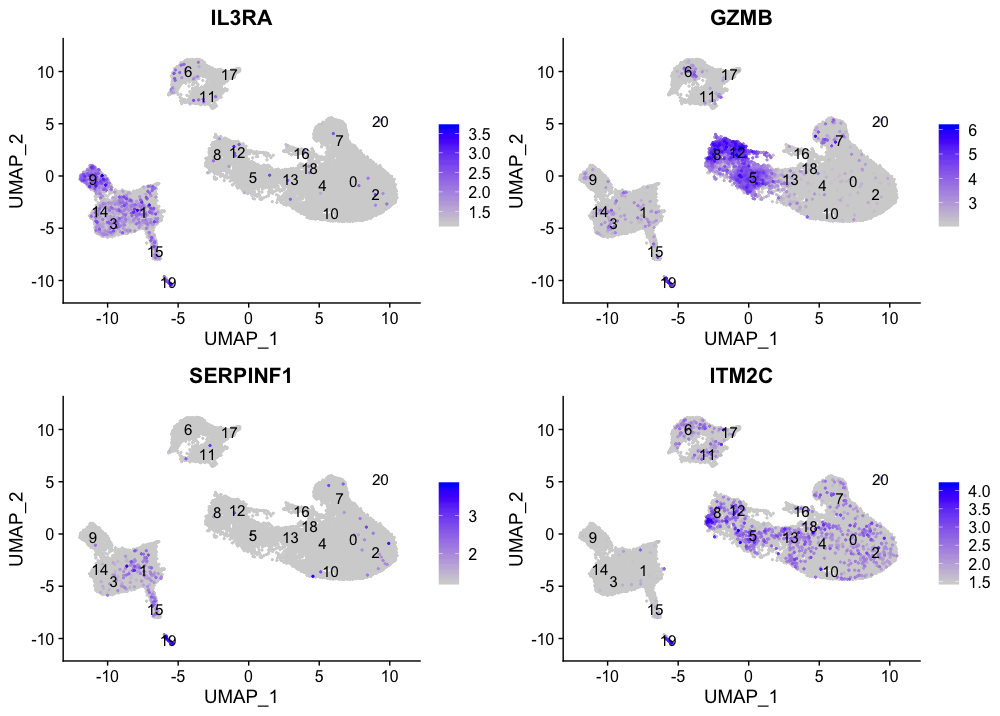 --- Another example: clustering of single cell data