class: center, middle, inverse, title-slide .title[ # Lecture 2: Sequence alignments and sequence search ] .subtitle[ ## BE4 4279 Bioinformatics SS 2024 ] .author[ ### January Weiner ] .date[ ### 2024-04-08 ] --- --- ## Sequences and sequence searches .pull-left[ * Nucleotide sequences: ``` 5'-ACCCGTAAAG-3' 5'-AAAAA...AAAA-3' 5'-TAA-3' (fig. on the right) ``` ] .pull-right[  ] --- ## Sequences and sequence searches * Amino acid sequences: ``` N-Ala-Val-Cys-C (fig. below) N-AVC-C (fig. below) ```  --- ## Sequences and sequence searches  --- ## Dot plots ✪ ``` A C G G T A A * * C * G * * T * A * * ``` --- ## Dot plots ``` Duplication A C G G T A A C G G T A A * * A * * C * C * G * * G * * T * T * A * * A * * C * G * * T * A * * ``` --- ## Dot plots ``` Duplication Insertion / Deletion A C G G T A A C G G T A A C G G G G G G T A A * * A * * A * * C * C * C * G * * G * * G * * * * * * T * T * T * A * * A * * A * * C * G * * T * A * * ``` --- ## Dot plots  --- ## Dot plots  --- --- ## Why do we have to search for sequences? * identify the organism from which a sequence comes from * find similar sequences * similarity -> common ancestry -> common function * understand the evolution of organisms (or viruses) * technical reasons: PCR, RNA-Seq etc. --- ## Homology, common ancestry and function ✪ * Homology: identity by descent -> if and only if there is a common ancestor * We can determine homology only by considering *phylogeny* * Homologous sequences often have similar functions, but exceptions are aplenty -- * Similarity: something we can easily calculate with a computer by doing an *alignment* * Similarity may indicate homology, but is not the same * Homologous sequences may not be very similar (e.g. large evolutionary distances) * Similar sequences (esp. short) may be result of chance, convergence or structural constraints (e.g. coiled-coil structures) -- * When we calculate the similarity between two sequences, we need some sort of statistics to measure similarity (e.g., whether sequences are very similar or really different) --- ## More on homology ✪ .pull-left[  ] .pull-right[ There are specific types of homology: * **orthology**: sequences are created by a speciation event. For example, alpha hemoglobin in humans and chimps * Very often, orthologous sequences have similar functions ] -- .pull-right[ * **paralogy**: sequenes are created by a duplication event in the genome. E.g., human alpha hemoglobin and human beta hemoglobin * Very often, paralogs have different function, for example due to neofunctionalization or subfunctionalization ] More on these topics later. --- ## If sequences are similar, are they homologous? ✪ * Similarity is a good indicator of homology * *Lack of similarity* is not a good indicator of *lack of homology* * To know for sure, you need to dive into phylogenetic reconstructions --- ## Why do we need to make alignments? ✪ Sequences always differ: * evolution -> mutations * post-processing (e.g. transcript isoforms) * sequencing errors => you cannot search by simple "Find"! --- ## Sequence alignments ✪ Examples of alingments of sequences `ACTTGA` and `ACCTGGA` ``` ACTTG-A ACTT-GA AC-TTG-A ---ACTTGA ACTTGA------- || || | || | || || | | | | || ACCTGGA ACCTGGA ACCT-GGA ACC--TGGA ------ACCTGGA ``` This is not a correct alignment (but may make sense in a different context): ``` ACTTG--A || || | ACCTG-GA ``` --- ## Do not confuse alignments with complementary sequences .pull-left[ Alignment: ``` 5'-ACTTG-A-3' || || | 5'-ACCTGGA-3' ``` ] .pull-right[ Complementary sequence: ``` 5'-ACTTGGA-3' ||||||| 3'-TGAACCT-5' ``` ] --- ## Scoring an alignment .pull-left[ * Which alignment is correct? * What makes an alignment better? * How do we compare alignments? ] .pull-right[ Which one is better? ``` ACTTG-A ---ACTTGA || || | | || ACCTGGA ACC--TGGA ``` ] ??? A good alignment reflects evolutionary history. Better: parsimony principle: each deletion is an event, each mismatch is an event. Find the lowest number of events. --- ## Scoring an alignment .pull-left[ * Maximize matches, minimize gaps * Simplest scoring: * each match receives a score * mismatches receive a lower score than matches between identical residues * gaps receive penalties ] -- .pull-right[ Example scoring: * match: +2 * mismatch: 0 * gap: -1 ``` ACTTG-A ---ACTTGA || || | | || ACCTGGA ACC--TGGA ``` ] ??? We will talk more about scores when we come to scoring matrices --- ## Number of possible alignments .pull-left[ The number of possible alignments is staggering! For two sequences of length `\(n\)` and `\(m\)`, respectively, the number of possible alignments is `$$A(n, m) = \frac{(n + m)!}{m!k!} \approx \frac{2^{2n}}{\sqrt{2 \cdot \pi \cdot n}}$$` ] .pull-right[ <!-- --> ] .footnote[*Eddy, Sean R. "What is dynamic programming?." Nature biotechnology 22.7 (2004): 909-910.*] --- ## Needleman-Wunsch algorithm * Possibly the most famous algorithm in bioinformatics * Still used if you want to have an exact alignment * Go on, try to implement it! --- ## Alignments as paths in the matrix <!-- --> --- ## Alignments as paths in the matrix <!-- --> --- ## Alignments as paths in the matrix <!-- --> --- ## Alignments as paths in the matrix <!-- --> --- ## Alignments as paths in the matrix <!-- --> --- ## Alignments as paths in the matrix <!-- --> --- ## Alignments as paths in the matrix <!-- --> --- ## Alignments as paths in the matrix <!-- --> --- ## Alignments as paths in the matrix <!-- --> --- ## Alignments as paths in the matrix <!-- --> --- ## Alignments as paths in the matrix <!-- --> --- ## Alignments as paths in the matrix <!-- --> --- ## Alignments as paths in the matrix <!-- --> --- ## Step 1: create a score matrix <!-- --> --- ## Step 2: calculate edit operations * "Moving" horizontally or vertically means including a gap, hence: gap penalty!) – e.g. -1 ``` A | C | T ... -------------- A| -> | A C T ... -------------- | C| | | | ... A - .... ``` * "Moving" diagonally means we are getting the score in the matrix (here: 0 or 1) --- ## Step 2: calculate edit operations --- ## Step 2: calculate edit operations <!-- --> --- ## Step 2: calculate edit operations <!-- --> --- ## Step 2: calculate edit operations <!-- --> --- ## Step 2: calculate edit operations <!-- --> --- ## Step 2: calculate edit operations --- ## Step 2: calculate edit operations <!-- --> --- ## Step 2: calculate edit operations <!-- --> --- ## Step 2: calculate edit operations <!-- --> --- ## Step 2: calculate edit operations <!-- --> --- ## Step 2: calculate edit operations --- ## Step 2: calculate edit operations <!-- --> --- ## Step 2: calculate edit operations <!-- --> --- ## Step 2: calculate edit operations <!-- --> --- ## Step 2: calculate edit operations <!-- --> --- ## Step 2: calculate edit operations <!-- --> --- ## Step 2: calculate edit operations .pull-left[ <!-- --> ] .pull-right[ Note: if you add the scores along the arrows, you will get the score of the alignment! 1 + 1 + 1 - 1 + 1 + 1 = 4 Here the alignment: ``` ACC-GT ||| || ACCGGT ``` Five matches minus one gap = 4, indeed. ] --- ## Step 2: calculate edit operations .pull-left[ * Start with top left corner * proceed column-wise, then row-wise * For each cell, determine from which direction it is optimal to "get in" * Store the information * where did we came from * what was the optimal score ] .pull-right[  ] Pseudocode: ``` score <- matrix[ 0:n1, 0:n2 ] direction <- matrix[ 0:n1, 0:n2 ] for each row of score[] for each column of score[] top <- score[ row - 1, column ] left <- score[ row, column - 1 ] topleft <- score[ row - 1, column - 1 ] score[ row, column ] <- max(top, left, topleft) or 0 direction[ row, column ] <- which max(top, left, topleft) or 0 ``` --- ## Step 2: calculate edit operations <!-- --> --- ## Step 2: calculate edit operations <!-- --> --- ## Step 2: calculate edit operations <!-- --> --- ## Step 2: calculate edit operations <!-- --> --- ## Step 2: calculate edit operations <!-- --> --- ## Step 2: calculate edit operations <!-- --> --- ## Step 2: calculate edit operations <!-- --> --- ## Step 2: calculate edit operations <!-- --> --- ## Step 2: calculate edit operations <!-- --> --- ## Step 2: calculate edit operations <!-- --> --- ## Step 2: calculate edit operations <!-- --> --- ## Step 2: calculate edit operations <!-- --> --- ## Step 2: calculate edit operations <!-- --> --- ## Step 2: calculate edit operations <!-- --> --- ## Step 2: calculate edit operations <!-- --> --- ## Step 3: get the alignment * We now start from the *lower*, *right* corner * The score in the lower right corner is the score of the alignment * We *trace back* the alignment to the beginning --- ## Step 3: get the alignment <!-- --> --- ## Step 3: get the alignment <!-- --> --- ## Step 3: get the alignment <!-- --> --- ## Step 3: get the alignment <!-- --> ``` ## [1] "*" "d" "d" "d" "d" "t" "d" ## [1] "*" "d" "d" "d" "t" "d" "d" ``` --- ## Step 3: get the alignment <!-- --> ``` ## [1] "*" "d" "d" "d" "d" "t" "d" ## [1] "*" "d" "d" "d" "t" "d" "d" ``` --- ## Step 3: get the alignment <!-- --> ``` ## [1] "*" "d" "d" "d" "d" "t" "d" ## [1] "*" "d" "d" "d" "t" "d" "d" ``` --- ## Step 3: get the alignment <!-- --> ``` ## [1] "*" "d" "d" "d" "d" "t" "d" ## [1] "*" "d" "d" "d" "t" "d" "d" ``` --- ## Step 3: get the alignment 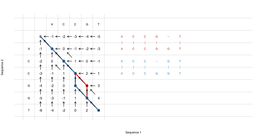<!-- --> ``` ## [1] "*" "d" "d" "d" "d" "t" "d" ## [1] "*" "d" "d" "d" "t" "d" "d" ``` --- ## That was hard, have a cat  --- ## Time complexity of NW ✪ `\(\sim O(n^2)\)` * polynomial time complexity "big O" notation – describes the type of relationship on an important parameter (like sequence length) rather than the precise relationship. It is more important to know how the performance *changes* when you increase the input than whether it will run 5 minutes or 10. --- ## Global vs local alignments * global: try to align the full length of both sequences * doesn't make sense if one sequence is a fragment of the other (think: searching for a gene in a genome) * often genes or proteins may share homologous regions only (e.g. multidomain proteins) * local: find the best sub-alignment – only a relevant fragment match ``` ACG-AG-GTGTGAAGGTCTAAAG--AGGCGA | | | |||||||| | | | | GCCCATAGAC--AAGGTCTA--GCCAAGAAA ``` vs. ``` AAGGTCTA |||||||| AAGGTCTA ``` --- ## Smith-Waterman algorithm Basically identical to NW, but: * set all negative scores to 0 * find the position in the matrix with the highest score and start from there --- ## Different gap penalties ``` AAGGGGTCTA AAGGGGTCTA |||| |||| ||| | |||| AAGG--TCTA AAG-G-TCTA ``` Same score, but different number of evolutionary events. Solution: introduce a higher gap opening penalty to differentiate these two situations. * gap opening penalty (e.g. 10) * gap extension penalty (e.g. 1) --- ## Different gap penalties High gap opening penalty: ``` HBA_HUMAN 1 MVLSPADKTNVKAAWGKVGAHAGEYGAEALERMFLSFPTTKTYFPHFDLS 50 |.|:..::|.:.:.|.|:...|...|.|.|||:|||.|.||||||||||. HBAZ_HUMAN 1 MSLTKTERTIIVSMWAKISTQADTIGTETLERLFLSHPQTKTYFPHFDLH 50 ``` Low gap opening penalty (equal to gap extension penalty) ``` HBA_HUMAN 1 MVLSPADKTN--VKAAWGKVGAHAGE-YGAEALERMFLSFPTTKTYFPHF 47 |.|:..::| | :.|.|:...| : .|.|.|||:|||.|.|||||||| HBAZ_HUMAN 1 MSLTKTERT-IIV-SMWAKISTQA-DTIGTETLERLFLSHPQTKTYFPHF 47 ``` --- ## The BLAST algorithm BLAST – Basic Local Alignment Search Tool 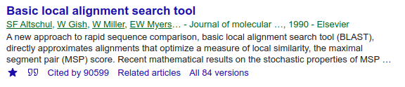  --- ## The BLAST algorithm 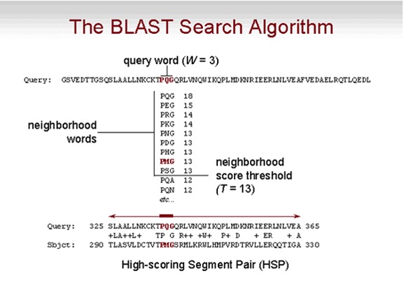 --- ## The BLAST algorithm * Advantage: `\(O(n)\)` – linear time complexity * Compromise between speed and sensitivity * Heuristic, not exact * Primary output: HSP, high scoring segment pairs (possibly multiple per sequence pair) --- ## Important BLAST parameters * Type of BLAST (which program) * Database (more on that tomorrow) * Word size (lower word size = slower but more sensitive) * Filter low complexity regions (e.g. repeats) --- ## BLAST E-value * Expected number of HSP's which have a score equal or better to the given result `\(E = m\cdot n\cdot 2^{-S'}\)` where `\(S'\)` is a normalized score and `\(m\)` and `\(n\)` are sequence lengths. `\(S' = \frac{\lambda S - \log{K}}{\log 2}\)` where S is the raw score ??? S depends on the scoring system, S' does not --- ## Guide to interpret E values: For protein sequences of moderate length: * `\(E < 10^{-100}\)` Practically identical * `\(10^{-100} < E < 10^{-50}\)` Almost identical * `\(10^{-50} < E < 10^{-10}\)` Closely related * `\(10^{-10} < E < 1\)` Unclear * `\(E > 1\)` Likely nothing * `\(E > 10\)` Nothing --- --- ## Burrow-Wheeler Aligner ✪ * BLAST is good for finding a long sequence against a database of billions of sequences * In second generation sequencing, we need to align quickly millions or billions of short (~ 50-200 nt) sequences against a genome with billions of nucleotides, but the alignments are almost perfect The BWA algorithm is based on the Burrow-Wheeler Transform (BWT) which allows quickly looking up short sequences in a genome --- ## BWA algorithm (overview): * Create the BWT of the genome * Create an index that allows fast searching of the genome --- ## BANANA genetics We will use the string `BANANA` to represent our genome. We will try to find the string `NANA` in the genome. --- * naive search * suffix search * BWA search --- ## Naive search We go from beginning to end, and each time we try to find a match: Search: `NANA` in `BANANA` * Go to `B`. Is it a match? No. continue. * Go to `A`. Is it a match? No. continue. * Go to `N`. Is it a match? Yes. * Match the `A` from `NANA`. Does it work? if yes, continue checking. If no, abort and continue searching in the genome. Time complexity: `\(O(m\times n)\)`. This is too slow! --- ## Suffixes and Prefixes ✪ **pre**fix <- this is a prefix confu**sion** <- this is a sufix Suffix search: build a database of suffixes --- `BANANA` -> `BANANA$` The `$` denotes end of our genome. When sorting alphabetically, we put it before any other characters. 1. Create all possible suffixes. 2. Sort suffixes alphabetically. --- ``` Suffix Pos BANANA$ 0 ANANA$ 1 NANA$ 2 ANA$ 3 NA$ 4 A$ 5 ``` --- ``` Suffix Pos BANANA$ 0 A$ 5 ANANA$ 1 ANA$ 3 NANA$ 2 -> ANANA$ 1 ANA$ 3 BANANA$ 0 NA$ 4 NA$ 4 A$ 5 NANA$ 2 ``` Now we can search using efficient searching algorithms, because the index is sorted. --- ## Suffix search Time complexity: `\(O(\log{n})\)`. This is much better than naive search, but the memory requirements are huge: you need to build a suffix array of the whole human genome, this is gigantic! --- ## BWT algorithm ``` unsorted sorted BANANA$ $BANANA A ANANA$B A$BANAN N NANA$BA ANA$BAN N ANA$BAN -> ANANA$B -> B NA$BANA BANANA$ $ A$BANAN NA$BANA A $BANANA NANA$BA A ``` --- ## BWT algorithm BANANA -> ANNB$AA This is more efficient to store. For example: BWT compression `peter_piper_picked_a_peck_of_pickled_peppers_a_peck_of _pickled_peppers_peter_piper_picked_if_peter_piper_picked _a_peck_of_pickled_peppers_wheres_the_peck_of_pickled_ peppers_peter_piper_picked` `\(\rightarrow\)` `ddsddkkkkaeaaddddsfsrrrrffffrrrrss___eeeeiiiiiiiieeeeeeeehpp ppkkkkllllpppppppptttthpppprppppiooootwpppppppp_pppp cccccccccccckkkk____________iiiipppp_______________eee eeeeeeeeeeeeeerrrereeee__` `\(\rightarrow\)` `2d1s3k1a1e2a4d1s1f1s4r4f2s3_4e8i8e1h4p4k4l8p4t1h4p1r4p1i4o1t1w8p1_4p12c4k12_4i4p12_16e3r1e1r4e2_` (much shorter!) --- ## BWT algorithm The real snag is that we can *reverse* this transform! (if we simply sorted all characters, we would not be able to do it) `$$iBWT(BWT(T)) = T$$` iBWT - inverse Burrow-Wheeler Transform BANANA -> ANNB$AA -> BANANA --- ## BWT algorithm ``` ......A $.....A $B....A $BANANA ......N A.....N A$....N A$BANAN ......N A.....N AN....N ANA$BAN ......B -> A.....B -> AN....B ... ANANA$B ......$ B.....$ BA....$ BANANA$ ......A N.....A NA....A NA$BANA ......A N.....A NA....A NANA$BA ``` --- ## BWA aligner That actually was simple; the BWA is more complex. However, it builds upon BWT to create an index of the genome. * BWA index is *much* smaller than the suffix array * **but** we can use the BWT to search for suffixes with a clever trick! * without getting into details, we need to also store some additional information (FM index), which allows us to use the BWT as a suffix array and directly look up any sequence --- # References <a name=bib-altschul1990basic></a>[Altschul, S. F., W. Gish, W. Miller, et al.](#cite-altschul1990basic) (1990). "Basic local alignment search tool". In: _Journal of molecular biology_ 215.3, pp. 403-410. <a name=bib-eddy2004dynamic></a>[Eddy, S. R.](#cite-eddy2004dynamic) (2004). "What is dynamic programming?" In: _Nature biotechnology_ 22.7, pp. 909-910.